Week 5 - Genetic Algorithm

Introduction:

The genetic algorithm (GA) is a search and optimization technique inspired by the process of natural selection and evolution. It is commonly used to solve complex optimization problems where traditional methods may be inefficient or infeasible. In this report, we will provide a conceptual explanation of genetic algorithms and discuss the syntax for implementing a GA in MATLAB.

Concept:

The genetic algorithm mimics the principles of natural selection, which involves the survival of the fittest and the passing of favourable traits from one generation to the next. GA operates on a population of potential solutions, where each solution represents a set of parameters or variables. The process involves iteratively evolving the population through several generations to find an optimal or near-optimal solution.

1. Initialization: The GA starts by randomly generating an initial population of potential solutions. Each solution is represented as a chromosome or a string of values, which can be binary, integer, or real-valued.
2. Fitness Evaluation: A fitness function is defined to evaluate the performance or suitability of each individual in the population. The fitness function assigns a fitness value to each chromosome based on how well it solves the problem at hand. This evaluation guides the selection of individuals for reproduction in the next steps.
3. Selection: The selection process simulates the survival of the fittest. Individuals with higher fitness values have a higher chance of being selected as parents for the next generation. Various selection methods can be used, such as roulette wheel selection, tournament selection, or rank-based selection.
4. Reproduction: Selected individuals are used to create offspring for the next generation through crossover and mutation operations. Crossover involves combining genetic information from two parents to create new offspring, mimicking genetic recombination. Mutation introduces small random changes in the offspring's genetic information to explore new regions of the search space.
5. Replacement: The new offspring, along with some individuals from the current generation, form the population for the next generation. The replacement strategy determines which individuals are preserved and which ones are replaced. Elitism, for example, keeps the best individuals from the current generation in the next generation to ensure the preservation of good solutions.
6. Termination: The GA iteratively repeats steps 2 to 5 until a termination condition is met. This condition can be a maximum number of generations, reaching a satisfactory fitness value, or a certain level of convergence.

Syntax for the 'ga' function in MATLAB:

1. x = ga(fun, nvars): Finds a local unconstrained minimum x to the objective function fun. nvars specifies the dimension (number of design variables) of fun.
2. x = ga(fun, nvars, A, b): Finds a local minimum x to fun, subject to linear inequalities A*x ≤ b.
3. x = ga(fun, nvars, A, b, Aeq, beq): Finds a local minimum x to fun, subject to linear equalities Aeq*x = beq and linear inequalities A*x ≤ b.
4. x = ga(fun, nvars, A, b, Aeq, beq, lb, ub): Defines lower bounds lb and upper bounds ub on the design variables x, so that a solution is found in the range lb ≤ x ≤ ub.
5. x = ga(fun, nvars, A, b, Aeq, beq, lb, ub, nonlcon): Subjects the minimization to the constraints defined in nonlcon, which represents nonlinear inequalities and equalities. nonlcon accepts x and returns vectors C and Ceq.
6. x = ga(fun, nvars, A, b, Aeq, beq, lb, ub, nonlcon, options): Minimizes with the optimization parameters specified in the options object, replacing the default parameters.
7. x = ga(fun, nvars, A, b, [], [], lb, ub, nonlcon, IntCon): Requires the variables listed in IntCon to take integer values.
8. x = ga(problem): Finds the minimum for problem, where problem is a structure containing the necessary inputs.
9. [x, fval] = ga(___ ): Returns the value of the fitness function at x as fval in addition to the optimal solution x.
10. [x, fval, exitflag, output] = ga(___): Returns exitflag, an integer identifying the termination reason, and output, a structure containing information about the algorithm's performance.
11. [x, fval, exitflag, output, population, scores] = ga(___ ): Also returns the final population population and their corresponding scores scores.

Main code:

% Genetic Algorithm

clear all
close all
clc

% search space inputs

x = linspace(0,1,200);
y = linspace(0,1,200);

cases = 50;

% creating a 2D mesh
[xx,yy] = meshgrid(x,y);

%Evaluating Stalagmite function
for i = 1:length(xx)
    for j = 1:length(yy)

        input_value(1)=xx(i,j);
        input_value(2)=yy(i,j);

        f(i,j) = stalagmite(input_value);

    end
end
surfc(x,y,f)

% Study1- Unbounded statistic
tic
for i = 1:cases

    [input, fopt1(i)] = ga(@stalagmite, 2);
    xopt1(i) = input(1);
    yopt1(i) = input(2);

end


study_time_1 = toc

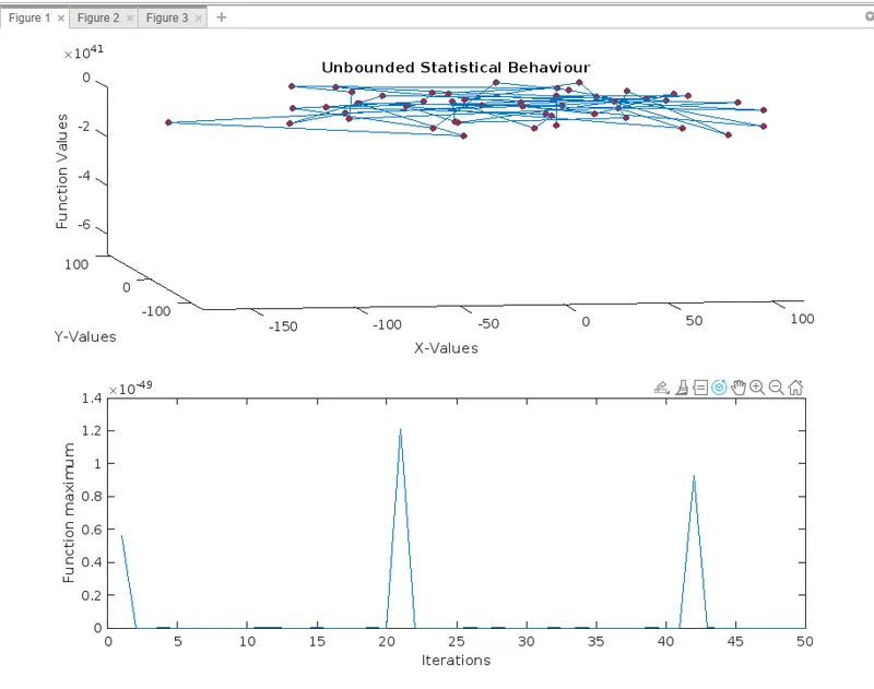
figure(1)

    subplot(2,1,1)
    hold on

    surfc(x,y,-f)
    xlabel('X-Values');
    ylabel('Y-Values');
    zlabel('Function Values');
    shading interp
    plot3(xopt1,yopt1,fopt1,'marker','o','markersize',5,'markerfacecolor','r');
    title('Unbounded Statistical Behaviour');

    subplot(2,1,2)
    plot(fopt1)
    hold off
    xlabel('Iterations');
    ylabel('Function maximum');

    
%Study2 - upper and lower bound
tic
for i = 1:cases

    [input2, fopt2(i)] = ga(@stalagmite, 2,[],[],[],[],[0;0],[1;1]);
    xopt2(i) = input2(1);
    yopt2(i) = input2(2);

end

study_time_2 = toc
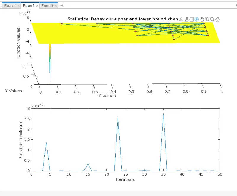
figure(2)

    subplot(2,1,1)
    hold on

    surfc(x,y,-f)
    xlabel('X-Values');
    ylabel('Y-Values');
    zlabel('Function Values');
    shading interp
    plot3(xopt2,yopt2,fopt2,'marker','o','markersize',5,'markerfacecolor','r');
    title('Statistical Behaviour-upper and lower bound change');

    subplot(2,1,2)
    plot(fopt2)
    hold off
    xlabel('Iterations');
    ylabel('Function maximum');

%Study3 - upper and lower bound
options = optimoptions('ga');
options = optimoptions(options,'PopulationSize',200);

tic
for i = 1:cases

    [input3, fopt3(i)] = ga(@stalagmite, 2,[],[],[],[],[0;0],[1;1],[],[],options);
    xopt3(i) = input2(1);
    yopt3(i) = input2(2);

end

study_time_3 = toc

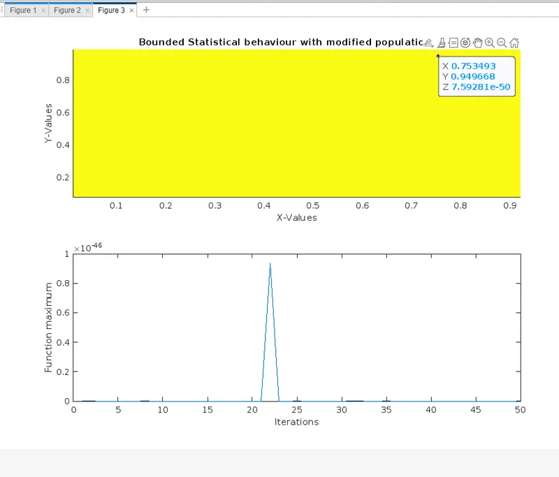
figure(3)

    subplot(2,1,1)
    hold on

    surfc(x,y,-f)
    xlabel('X-Values');
    ylabel('Y-Values');
    zlabel('Function Values');
    shading interp
    plot3(xopt3,yopt3,fopt3,'marker','o','markersize',5,'markerfacecolor','r');
    title('Bounded Statistical behaviour with modified population size');

    subplot(2,1,2)
    plot(fopt3)
    hold off
    xlabel('Iterations');
    ylabel('Function maximum');

 T_study_time = study_time_1+study_time_2+study_time_3

Explanation:

• clear all, close all, clc: These commands clear the workspace, close all figures, and clear the command window.
• x = linspace(0,1,200): Creates a linearly spaced vector x with 200 points ranging from 0 to 1.
• y = linspace(0,1,200): Creates a linearly spaced vector y with 200 points ranging from 0 to 1.
• cases = 50: Specifies the number of cases for the study.
• [xx,yy] = meshgrid(x,y): Creates a 2D meshgrid using x and y vectors. This will be used for evaluating the function over the entire search space.

• 12-20: Evaluates the function stalagmite for each combination of xx and yy values and stores the results in the matrix f. This loop iterates over each point in the meshgrid and calculates the function value.
• 22-26: Plots the surface of the function using surfc with x, y, and f as inputs.

• tic: Starts a timer to measure the elapsed time.

• 32-41: Performs Study 1 - Unbounded statistic. It runs the genetic algorithm (GA) cases times and stores the optimal input, function value, and corresponding x and y

• study_time_1 = toc: Stops the timer and assigns the elapsed time to the variable study_time_1.

• 47-57: Plots the results of Study 1. The subplot(2,1,1) command creates a 2x1 grid of subplots and selects the first subplot. It plots the function surface, overlays the optimal points, and labels the axes. The subplot(2,1,2) command selects the second subplot and plots the function maximum versus iterations.

• tic: Starts the timer for Study 2.

• 65-74: Performs Study 2 - Upper and lower bound change. It runs the GA with the specified lower and upper bounds for cases times and stores the optimal input, function value, and corresponding x and y

• study_time_2 = toc: Stops the timer and assigns the elapsed time to the variable study_time_2.

• 80-90: Plots the results of Study 2 similar to Study 1.

• options = optimoptions('ga'): Creates an options object for the GA with default settings.
• options = optimoptions(options,'PopulationSize',200): Modifies the options object to set the population size to 200.
• tic: Starts the timer for Study 3.

• 102-111: Performs Study 3 - Bounded statistical behavior with modified population size. It runs the GA with the specified lower and upper bounds and the modified population size for cases It stores the optimal input, function value, and corresponding x and y values.

• study_time_3 = toc: Stops the timer and assigns the elapsed time to the variable study_time_3.

• 117-127: Plots the results of Study 3 similar to Study 1 and Study 2.
• T_study_time = study_time_1 + study_time_2 + study_time_3: Calculates the total study time by summing the elapsed times of the three studies.

Function code:

%Function stalagmite

function [f] = stalagmite(input_value)

pi=3.14;

    f_1x = sin(5.1*pi*input_value(1)+ 0.5).^6;
    f_1y = sin(5.1*pi*input_value(2)+ 0.5).^6;
    f_2x = exp(-4*log((2)*(input_value(1)-0.0667).^2/(0.64)));
    f_2y = exp(-4*log((2)*(input_value(2)-0.0667).^2/(0.64)));

    f = -(f_1x .* f_1y .* f_2x .* f_2y);
end

Explanation:

The code provided defines the stalagmite function, which takes an input value as an argument and returns the corresponding function value.

• function [f] = stalagmite(input_value): This line defines the function named stalagmite that takes an input value as an argument and returns the function value f.
• pi = 3.14;: Assigns the value 3.14 to the variable pi. Note that MATLAB provides the built-in constant pi, so this line is not necessary.

• 5-6: Computes f_1x and f_1y by applying the sine function to the input values. The input values are multiplied by 1*pi and added 0.5 before taking the power of 6.
• 8-9: Computes f_2x and f_2y using exponential and logarithmic operations. The input values are subtracted by 0667, squared, and scaled before being used in the logarithmic expression.

• f = f_1x .* f_1y .* f_2x .* f_2y;: Calculates the overall function value f by multiplying the individual components f_1x, f_1y, f_2x, and f_2y element-wise.

Outputs:

Errors faced:

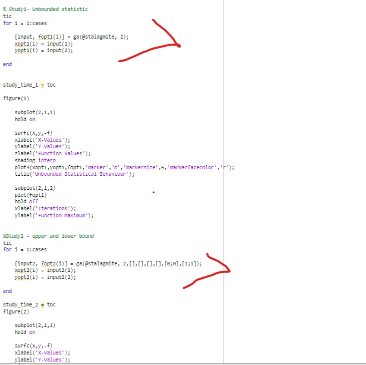
In this piece of code i had not changed the from fopt1,xopt1 and yopt1 which should be replaced by fopt2,xopt2 and yopt2.

Error found and rectified.

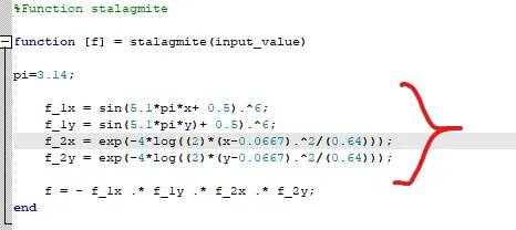
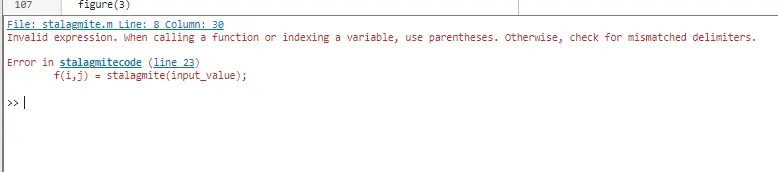
Here I had not assigned any values for x and y, instate it should be input_value(1), input_value(2).

Error found and rectified.

GA function not working in octave. Switched to online matlabs and it works fine.

NOTE: The stalagmite graphs are not showing properly but the solution in correct. I have cross-checked with a skill-lync mentor regarding the same. She informed this may be because I am using the online version.

References:

https://www.youtube.com/watch?v=96-u9s6D16k

https://www.youtube.com/watch?v=1i8muvzZkPw

https://in.mathworks.com/help/gads/ga.html