Week 5 - Genetic Algorithm

AIM

• Optimization Method using MATLAB
• Genetic Algorithm

THEORY

Optimization

Optimization is a decision-making process, it helps to find the best results under a set of prioritized criteria or constraints. It is a procedure which is executed iteratively by comparing various solutions till an optimum or satisfactory solution is found. These include maximizing factors such as productivity, strength, reliability, efficiency, utilization, etc.

Techniques available to perform Optimization

Deterministic Method

They use specific rules for moving one solution to another. In this technique, the output of the model is fully determined by the parameter values and the initial conditions. Example - Stress analysis of the component.

Stochastic Method

These are gaining popularity due to certain properties which deterministic algorithms do not possess. Stochastic models possess some inherent randomness, it is a probabilistic approach.

The procedure followed by any Optimization process

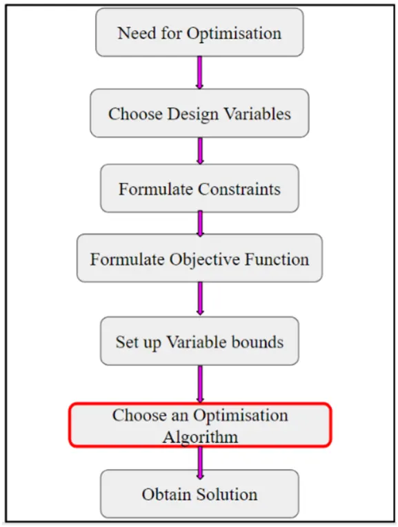
Genetic Algorithm

The genetic algorithm is one of the optimization processes. A genetic Algorithm (GA) is a search–based optimization technique based on the principles of Genetics and natural selection. It is frequently used to find optimal or near-optimal solutions.

The genetic algorithm is a method for solving both constrained and unconstrained optimization problems that are based on natural selection, the process that drives biological evolution. The genetic algorithm repeatedly modifies a population of individual solutions. At each step, the genetic algorithm selects individuals from the current population to be parents and uses them to produce children for the next generation. Over successive generations, the population “evolves” toward an optimal solution. The genetic algorithm can address problems of mixed integer programming, where some components are restricted to be integer-valued.

How does GA work?

The genetic algorithm uses three main types of rules at each step to create the next generation from the current population:

• Selection rules select the individuals, called parents that contribute to the population of the next generation. The selection is generally stochastic and can depend on the individuals’ scores.
• Crossover rules combine two parents to form children for the next generation.
• Mutation rules apply random changes to individual parents to form children.

The genetic algorithm differs from a classical, derivative-based, optimization algorithm in two main ways, as summarized in the following table:

Classical Algorithm	Genetic Algorithm
Generates a single point at each iteration. The sequence of points approaches an optimal solution.	Generates a population of points at each iteration. The best point in the population approaches an optimal solution.
Selects the next point in the sequence by a deterministic computation.	Selects the next population by computation which uses random number generators.
Typically converges quickly to a local solution.	Typically takes many function evaluations to converge. May or may not converge to a local or global minimum.

Where GA is used?

Genetic Algorithms are primarily used in optimization problems of various kinds, but they are frequently used in other application areas as well.

The areas in which GA are frequently used are listed below:

• Optimization – Genetic Algorithms are most commonly used in optimization problems wherein we have to maximize or minimize a given objective function value under a given set of constraints.
• Economics – GA is also used to characterize various economic models like the cobweb model, game theory equilibrium resolution, asset pricing, etc.
• Neural Networks – GA are also used to train neural networks, particularly recurrent neural networks.
• Image Processing – GA is used for various digital image processing (DIP) tasks as well as dense pixel matching.

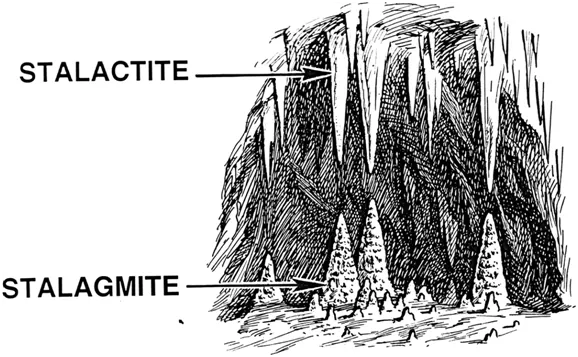
Stalagmite Function

A stalagmite function generally refers to the function with which we are generating values over a stalagmite kind of surface for finding out the local and global maxima and minima of that particularly given function.

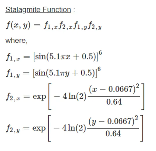
FUNCTION CODE:

function [f] = stalagmite(input_vector)

f1x = (sin((5.1*pi).*input_vector(1) + 0.5)).^6;
f1y = (sin((5.1*pi).*input_vector(2) + 0.5)).^6;

f2x = exp((((input_vector(1) - 0.0667).^2)/0.64).*(-4*log(2)));
f2y = exp((((input_vector(2) - 0.0667).^2)/0.64).*(-4*log(2)));

f = -f1x*f1y*f2x*f2y;

end

Main Body :-

• Firstly creating the mesh from the two vectors which will be acting as a search space to find the maxima of the function.
• Creating the mesh of these two vectors using the 'mesh' command and defining the number of iterations as 'num_cases' to iterate the values of the optimum values of the function.
• Now calculating the values of fitness function at each point of the mesh grid formed.
• Now creating the values of fitness function at each point of the mesh grid formed.
• Now creating its surface through 'surfc' command which will also provide the contour of the generated surfaces.
• While using surfcapplying the -ve sign to the function will generate the surface upside down which will be quite good to get the maxima of the function, as it will provide positive value for the maxima using the -ve sign.

MAIN CODE:

close all
clear all
clc

% Defining our search space
x = linspace(0,0.6,150);
y = linspace(0,0.6,150);

% number of iterations
num_cases = 50;

% 2D mesh
[xx yy] = meshgrid(x, y);

% f = get_stalagmite(x,y);
for i = 1:length(xx)
    for j = 1:length(yy)
        input_vector(1) = xx(i,j);
        input_vector(2) = yy(i,j);
        f(i,j) = stalagmite(input_vector);
    end
end

tic
% Study 1 - Statistical behavior
for i = 1:num_cases
    [inputs, fopt(i)] = ga(@stalagmite, 2);
    xopt(i) = inputs(1);
    yopt(i) = inputs(2);
end

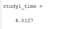
study1_time = toc

% unbounded 
figure(1)
subplot(2,1,1)
surfc(x,y,-f)
hold on 
shading interp 
plot3(xopt,yopt,-fopt,'marker','o','MarkerSize',5,'MarkerFaceColor','r')
title('Unbounded Inputs')
subplot(2,1,2)
plot(-fopt)
xlabel('Iterations')
ylabel('Function Minimum')

tic
% Study 2 - Statistical behaviour - with upper and lower bounds
for i = 1: num_cases
    [inputs, fopt(i)] = ga(@stalagmite,2,[],[],[],[],[0;0],[1;1]);
    xopt(i) = inputs(1);
    yopt(i) = inputs(2);
end

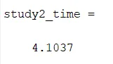
study2_time = toc

% bounded
figure(2) 
subplot(2,1,1)
surfc(x,y,-f)
hold on
shading interp
plot3(xopt,yopt,-fopt,'marker','o','MarkerSize',5,'MarkerFaceColor','r')
title('Bounded Inputs')
subplot(2,1,2)
plot(-fopt)
xlabel('Iterations')
ylabel('Function Minimum')

% Study 3 - increasing GA iterations
options = optimoptions('ga');
options = optimoptions(options,'PopulationSize',170);

tic
for i = 1:num_cases
    [inputs, fopt(i)] = ga(@stalagmite,2,[],[],[],[],[0;0],[1;1],[],[],options);
    xopt(i) = inputs(1);
    yopt(i) = inputs(2);
end

study3_time = toc

% Optimised
figure(3)
subplot(2,1,1)
surfc(x,y,-f)
hold on
shading interp
plot3(xopt,yopt,-fopt,'marker','o','MarkerSize',5,'MarkerFaceColor','r')
title('Optimized Inputs')
subplot(2,1,2)
plot(-fopt)
xlabel('Iterations')
ylabel('Function Minimum')

STEP BY STEP CODING PROCEDURE :-

1. First, Linspace command is used to define x & y with 150 elements between zero and 0.6 including the bounds.
2. Then num_cases is set which will be used as counter for iteration to 50
3. then a 2D grid is made using meshgrid command is created from x & y input tobe output to xx & yy
4. then for loop is used to solve the genetic algorithm for every element in the 2D mesh grid
5. the length of rows & column (which have equal length) are used as counters
6. then the input vector is declared as ga requires input vector which is each value in the mesh grid
7. then output of stalagmite function is stored in matrix
8. then tic command is used to start a timer
9. then for loop bounded by the number of iterations is formed
10. then ga code is entered for unbounded statistical study which have the following format :

[inputs, fopt] = ga(fun, nvars)

inputs represent the values of parameters x & y for which the function has the least value (fopt)

fun - the function tobe optimized, in this case stalagmite

nvars - the number of design variables, in this case only x & y are the variables tobe plotted

11. Then smallest (minimum) value of the function for each iteration is output & its x & y coordinates which are stored in seperate variables
12. then 'toc' command is used to stop the timer and the output is stored in study_time1
13. then figure1 is plotted by the following steps-
14. First subplot command is used to partition the plot window in order to draw more than one plot in the same window, two rows and one column are specified and then the position of each plot is selected
15. then hold on command is used to prevent plot for being removed
16. the surfc command is used to plot contour with xx & yy value from the mesh grid as input and negative optimum value is used because we need to maximize the function
17. then x,y,& z axis are labelled
18. then shading interp is used to smoothen the function plot and to remove the grid lines
19. then plot 3 command is used to plot a point in 3D, here it will plot- fopt because we need the maximum value of the function not the minimum
20. then the graph title is selected
21. then fopt value of the function is plotted on the second plot in the second row
22. then its x & y axis are labelled.
23. then the same study is made but this time it is bounded (has lower & upper limit) which requires the same commands and step excepts the ga command which have the following format :

[input, fopt] = ga(fun, nvars, A, b, Aeq, beq, lb, ub)

Inputs, fopt, fun & nvars are the same as study-1

A - Linear inequality constraints : real matrix, if there are none, then []

b - Linear inequality constraints : real vector, if there are none, then []

Aeq - Linear equality constraints - :- real matrix, if there are none, then []

beq - Linear equality constraints - real vector, if there are none, then []

lb - lower bounds, specified as a real vector or array

ub - upper bounds, specified as a real vector or array

24. the range of the genetic algorithm is bounded by introducing values for lower and upper bounds and hence the values of global maxima and the values of x & y will be within the defined search space in inputs
25. then increasing population size study was done which is the same as before but it had different ga code of :

[inputs, fopt] = ga(fun, nvars, A, b, Aeq, beq, lb, ub, nonlcon, IntCon, options)

inputs, fopt, fun and nvars, A, b, Aeq, beq, lb, ub are the same as study-1 and study -2 respectivelly

nonlcon - nonlinear constraints, specified as a function handle or function name. If there are none then []

IntCon - Integer variables, specified as a vector of positive integers, if there are none, then []

Options - Optimization options, specified as the output of optimoptions or a structure.

26. the range of the genetic algorithm is bounded as in study-2 but to improove the accuracy, the commands optimoptions is introduced to increase the Population Size
27. then total time is computed
28. then using fprintf command the results are printed in the command windows
29. then the study time is printed
30. then x, y coordinate of the maximum optimum values are printed
31. then the optimum values of the function (maximum value) is printed which is calculated from the (negative mean) of the all iterations of the output value and the negative sign is used to get the maximum value
32. then the study time of the whole 3 studies combined is printed.

OUTPUT

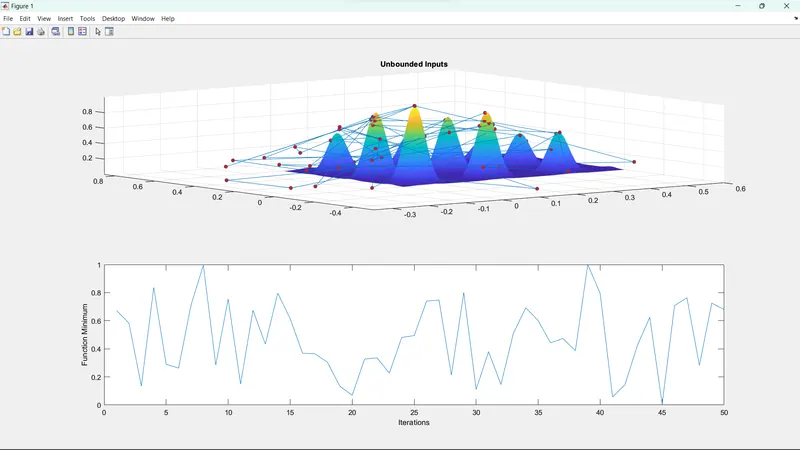
• The first study ( Unbounded )

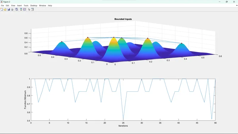
• The second study (Bounded)

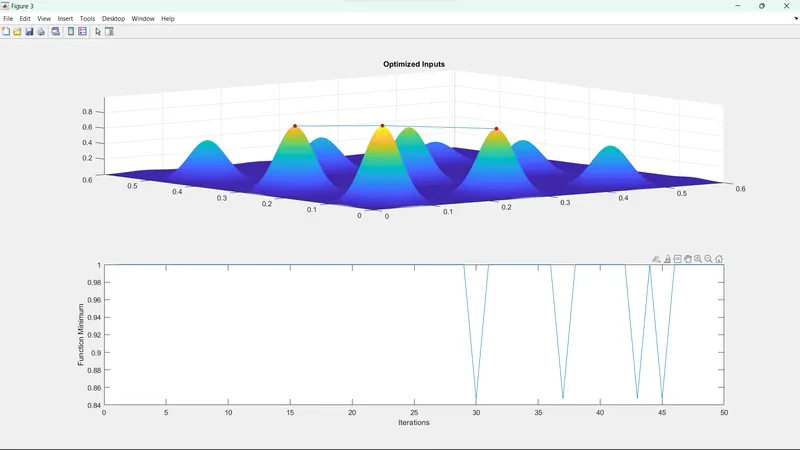
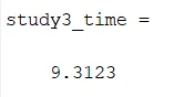
• The third study (Optimized)

OUTPUT EXPLANATION

The above results show that the bounded samples with population size have an accurate solution. This is because the code shows the random samples which can start and end at random points.

To overcome the issue, the bounded samples method is used giving the lower and upper limits. (Therefore, it will take the values which are greater than the upper bound or less than the lower bound.)

This loop gives an output with different local maxima with bounded inputs. To conquer this problem, we need to increase the population size as it increases the probability to converge to a global maximum.

The global maximum of a function can be found by inverting the function. Find the minimum value of the inverted function, the negative of the minimum value will give the global maximum of the function.

REFERENCES

• https://in.mathworks.com/help/gads/what-is-the-genetic-algorithm.html
• https://towardsdatascience.com/introduction-to-genetic-algorithms-including-example-code-e396e98d8bf3?gi=6aafe4b48f5