Week 5 - Genetic Algorithm
GENETIC ALGORIYHM
OBJECTIVE:
To explain the concept of Genetic algorithm and its syntax and also to find the global maxima of the function.
GENETIC ALGORITHM:
A genetic algorithm (GA) is a method for solving both constrained and unconstrained optimization problems based on a natural selection process that mimics biological evolution. The algorithm repeatedly modifies a population of individual solutions. At each step, the genetic algorithm randomly selects individuals from the current population and uses them as parents to produce the children for the next generation. Over successive generations, the population "evolves" toward an optimal solution. You can apply the genetic algorithm to solve problems that are not well suited for standard optimization algorithms, including problems in which the objective function is discontinuous, nondifferentiable, stochastic, or highly nonlinear.
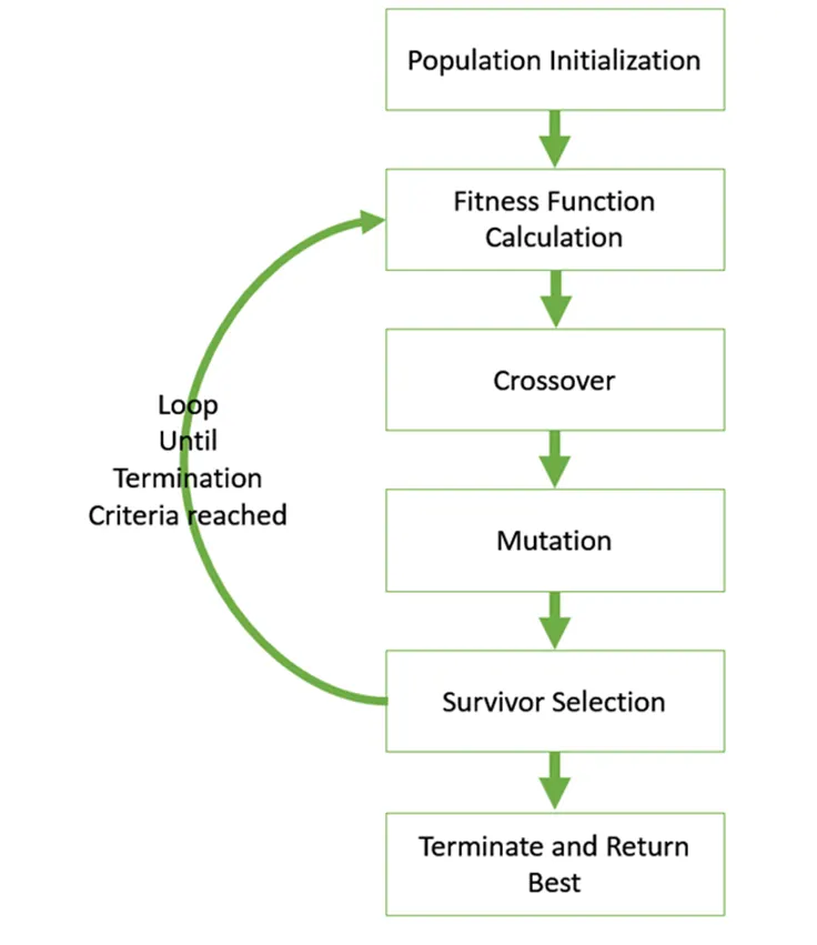
Fig. 1
Population − It is a subset of all the possible (encoded) solutions to the given problem. The population for a GA is analogous to the population for human beings except that instead of human beings, we have Candidate Solutions representing human beings.
Fitness Function − A fitness function simply defined is a function which takes the solution as input and produces the suitability of the solution as the output. In some cases, the fitness function and the objective function may be the same, while in others it might be different based on the problem.
Crossover - Crossover is the most vital stage in the genetic algorithm. During crossover, a random point is selected while mating a pair of parents to generate offspring.
There are 3 major types of crossovers.
- Single Point Crossover: A point on both parents’ chromosomes is picked randomly and designated a ‘crossover point’. Bits to the right of that point are exchanged between the two parent chromosomes.
- Two-Point Crossover: Two crossover points are picked randomly from the parent chromosomes. The bits in between the two points are swapped between the parent organisms.
- Uniform Crossover: In a uniform crossover, typically, each bit is chosen from either parent with equal probability.
Mutation - In a few new offspring formed, some of their genes can be subjected to a low random probability mutation. This indicates that some of the bits in the bit chromosome can be flipped. Mutation happens to take care of diversity among the population and stop premature convergence.
The Survivor Selection - The Survivor Selection Policy determines which individuals are to be kicked out and which are to be kept in the next generation. It is crucial as it should ensure that the fitter individuals are not kicked out of the population, while at the same time diversity should be maintained in the population.
Termination condition - The termination condition of a Genetic Algorithm is important in determining when a GA run will end. It has been observed that initially, the GA progresses very fast with better solutions coming in every few iterations, but this tends to saturate in the later stages where the improvements are very small. We usually want a termination condition such that our solution is close to the optimal, at the end of the run.
Usually, we keep one of the following termination conditions
- When there has been no improvement in the population for X iterations.
- When we reach an absolute number of generations.
- When the objective function value has reached a certain pre-defined value.
GA SYNTAX:
The genetic algorithm uses three main types of rules at each step to create the next generation from the current population:
x = ga(fun,nvars)
x = ga(fun,nvars,A,b)
x = ga(fun,nvars,A,b,Aeq,beq)
x = ga(fun,nvars,A,b,Aeq,beq,lb,ub)
x = ga(fun,nvars,A,b,Aeq,beq,lb,ub,nonlcon)
x = ga(fun,nvars,A,b,Aeq,beq,lb,ub,nonlcon,options)
x = ga(fun,nvars,A,b,[],[],lb,ub,nonlcon,IntCon)
x = ga(fun,nvars,A,b,[],[],lb,ub,nonlcon,IntCon,options)
x = ga(problem)
[x,fval] = ga(___)
[x,fval,exitflag,output] = ga(___)
[x,fval,exitflag,output,population,scores] = ga(___)
1. x = ga(fun,nvars) finds a local unconstrained minimum, x, to the objective function, fun. nvars is the dimension (number of design variables) of fun.
2. x = ga(fun,nvars,A,b) finds a local minimum x to fun, subject to the linear inequalities A*x ≤ b. ga evaluates the matrix product A*x as if x is transposed (A*x').
3. x = ga(fun,nvars,A,b,Aeq,beq) finds a local minimum x to fun, subject to the linear equalities Aeq*x = beq and A*x ≤ b. (Set A=[] and b=[] if no linear inequalities exist.) ga evaluates the matrix product Aeq*x as if x is transposed (Aeq*x').
4. x ga(fun,nvars,A,b,Aeq,beq,lb,ub) defines a set of lower and upper bounds on the design variables, x, so that a solution is found in the range lb ≤ x ≤ ub. (Set Aeq=[] and beq=[] if no linear equalities exist.)
5. x = ga(fun,nvars,A,b,Aeq,beq,lb,ub,nonlcon) subjects the minimization to the constraints defined in nonlcon. The function nonlcon accepts x and returns vectors C and Ceq, representing the nonlinear inequalities and equalities respectively. ga minimizes the fun such that C(x) ≤ 0 and Ceq(x) = 0. (Set lb=[] and ub=[] if no bounds exist.)
6. x = ga(fun,nvars,A,b,Aeq,beq,lb,ub,nonlcon,options) minimizes with the default optimization parameters replaced by values in options. (Set nonlcon=[] if no nonlinear constraints exist.) Create options using optimoptions.
7. x = ga(fun,nvars,A,b,Aeq,beq,lb,ub,nonlcon,Intcon) requires that the variables listed in IntCon take integer values.
8. x=ga(problem) finds the minimum for problem, where problem is a structure.
9. [x,fval] = ga(__) for any previous input arguments, also returns fval, the value of the fitness function at x.
10. [x,fval,exitflag,output] = ga(__) also returns exitflag, an integer identifying the reason the algorithm terminated, and output, a structure that contains output from each generation and other information about the performance of the algorithm.
11. [x,fval,exitflag,output,population,scores] = ga(__) also returns a matrix population, whose rows are the final population, and a vector scores, the scores of the final population.
WORKING OF GA:
The algorithm begins by creating a random initial population. The algorithm then creates a sequence of new populations. At each step, the algorithm uses the individuals in the current generation to create the next population.
To create the new population, the algorithm performs the following steps: Scores each member of the current population by computing its fitness value. These values are called the raw fitness scores.
Scales the raw fitness scores to convert them into a more usable range of values. These scaled values are called expectation values. Selects members, called parents, based on their expectation.
Some of the individuals in the current population that have lower fitness are chosen as elite. These elite individuals are passed to the next population. Produces children from the parents.
STALAGMITE FUNCTION:
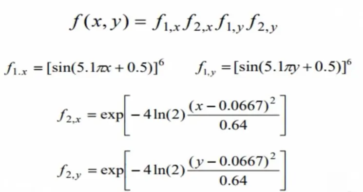
A stalagmite is an upward-growing mound of mineral deposits that have precipitated from water dripping onto the floor of a cave. The figures we get is in the shape of stalagmite so we use this name here. These formulas are represented in the below code.
The Parameters used in the solution(Program) of Genemtic Algorithm:
1.Surfc:
surfc function contours the plot under the surface plot. surfc(X, Y, Z) creates a three-dimensional surface plot with a contour plot underneath. A surface plot is a three-dimensional surface that has solid edge colors and solid face colors. The function plots the values in matrix Z as heights above a grid in the x-y plane defined by X and Y. The color of the surface varies according to the heights specified by Z.
2.Shading:
The shading function controls the color shading of surface and patch graphics objects. Shading flat each mesh line segment and face has a constant color determined by the color value at the endpoint of the segment or the corner of the face that has the smallest index or indices. Shading faceted flat shading with superimposed black mesh lines. This is the default shading mode. shading interp varies the color in each line segment and face by interpolating the colormap index or true color value across the line or face. shading(axes_handle,...) applies the shading type to the objects in the axes specified by axes_handle, instead of the current axes. Use single quotes when using a function form. For example:
shading(gca,'interp')
3.Plot3:
plot3(X, Y, Z) plots coordinates in 3-D space.
To plot a set of coordinates connected by line segments, specify X, Y, and Z as vectors of the same length.
To plot multiple sets of coordinates on the same set of axes, specify at least one of X, Y, or Z as a matrix and the others as vectors.
4.Optimoptions:
options = optimoptions(SolverName) returns a set of default options for the SolverName solver.
options = optimoptions(oldoptions,Name,Value) returns a copy of oldoptions with the named parameters altered with the specified values.
Tic- Toc:
tic works with the toc function to measure elapsed time. The 'tic' function records the current time, and the toc function uses the recorded value to calculate the elapsed time.
toc reads the elapsed time since the stopwatch timer started by the call to the tic function. MATLAB reads the internal time at the execution of the toc function and displays the elapsed time since the most recent call to the tic function without an output. The elapsed time is expressed in seconds
clear all
close all
clc


% Defining our space source
x = linspace(0,0.6,150);
y = linspace(0,0.6,150);
num_cases = 50;            % The Number of Iterations for the optimal generation


% creating a 2 Dimensional mesh
[xx,yy] = meshgrid(x,y);

% Evaluating the stalagmite function
for i = 1:length(xx)                  % FOR LOOP for xx source
    for j = 1:length(yy)              % FOR LOOP for yy source
        input_vector(1) = xx(i,j);
        input_vector(2) = yy(i,j);
        f(i,j) = stalagmite(input_vector);  % Allowing Stalagmite function
    end
end

figure(4)
surfc(xx,yy,-f)            % Three-dimensional surface plot with a contour plot undetneath
shading interp             % For control of surfece and patch graphic of object
[x,fval] = ga(@stalagmite,2);   % Plot Genetic algorithm
xlabel("x-axis")
ylabel("y-axis")
title("Stalagmite plot")

% study1 - statistical behaviour
tic                                % Tic Starts the Clock time for the function
for i = 1:num_cases
    [input,fopt(i)] = ga(@stalagmite,2);
    xopt(i) = input(1);
    yopt(i) = input(2);
end

study1_time = toc;                % Toc stops the timer and shows the end time

figure(1)
subplot(2,1,1)
hold on
surfc(xx,yy,-f)
shading interp
plot3(xopt,yopt,-fopt,'Marker','o','MarkerSize',5,'MarkerEdgeColor','r')  % plot co-ordinates in 3-d space
xlabel('x-axis')
ylabel('y-axis')
title('Unbounded inputs')
subplot(2,1,2)
plot(-fopt)                       % Plot of "fopt" space
xlabel('Iterations')
ylabel('Function Maximum')
shading interp


% study2 - statistical behaviour
tic                                  % Tic Starts the Clock time for the function
for i = 1:num_cases
    [input,fopt(i)] = ga(@stalagmite,2,[],[],[],[],[0;0],[0.6;0.6]);
    xopt(i) = input(1);
    yopt(i) = input(2);
end

study2_time = toc;                   % Toc stops the timer and shows the end time

figure(2)
subplot(2,1,1)
hold on
surfc(xx,yy,-f)
shading interp
plot3(xopt,yopt,-fopt,'Marker','o','MarkerSize',5,'MarkerEdgeColor','r')   % plot co-ordinates in 3-d space
xlabel('x-axis')
ylabel('y-axis')
title('Bounded inputs')
subplot(2,1,2)
plot(-fopt)                        % Plot of "fopt" space
xlabel('Iterations')
ylabel('Function Maximum')
shading interp


% study3 - statistical behaviour
options = optimoptions('ga');
options = optimoptions(options,'PopulationSize',170);

tic                            % Tic Starts the Clock time for the function
for i = 1:num_cases
    [input,fopt(i)] = ga(@stalagmite,2,[],[],[],[],[0;0],[0.6;0.6],[],[],options);
    xopt(i) = input(1);
    yopt(i) = input(2);
end

study3_time = toc;             % Toc stops the timer and shows the end time

figure(3)
subplot(2,1,1)
hold on
surfc(xx,yy,-f)
shading interp
plot3(xopt,yopt,-fopt,'Marker','o','MarkerSize',5,'MarkerEdgeColor','r')  % plot co-ordinates in 3-d space
xlabel('x-axis')
ylabel('y-axis')
title('Bounded inputs with modified population size')
subplot(2,1,2)
plot(-fopt)                  % Plot of "fopt" space
xlabel('Iterations')
ylabel('Function Maximum')
shading interp


global_maxima = -fopt;            % Global Maxima of Plot


Function program for Genetic Algorithm(Stalagmite function)

% Stalagmite function for genetic algorithm
% The stalagmite formula is distributed in form of as below

function[f] = stalagmite(input_vector)

x = input_vector(1);
y = input_vector(2);
f1x = (sin(5.1*pi*x + 0.5))^6;
f1y = (sin(5.1*pi*y + 0.5))^6;
f2x = exp(-4*log(2)*(x-0.0667)^2/0.64);
f2y = exp(-4*log(2)*(y-0.0667)^2/0.64);
f = -(f1x*f2x*f1y*f2y);
end
OUTPUT AND RESULTS:
Simple Stalagmite and genetic algorithm plot
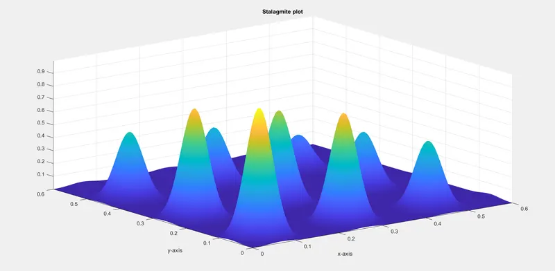
The above Fig.(picture) shows the stalagmite shape(plot).
Study time 1 - statical behaviour (Unbounded Inputs) sample output
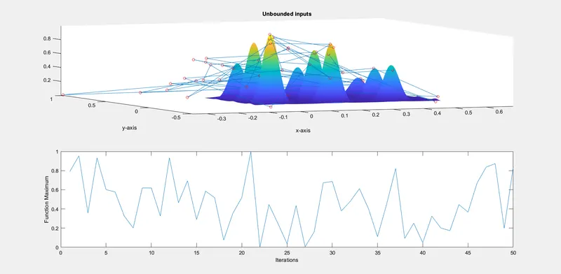
The above result shows the Unbounded Inputs included points. In the above the random number of inputs are took from number of cases. The stalagmite function is harder to find the maximum point in the above figure.
Study time 2 - statical behaviour (Bounded Inputs) sample output
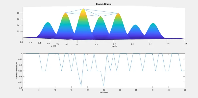
In the above result Bounded inputs are included. The provided inputs not in random but applied as Lower bound and Upper bound. So the plot bit clear, but the maximum point is not delarable. Hence the plot need to smoother more.
Study time 3 - statical behaviour (Bounded Inputs with Modified Population Size) sample output
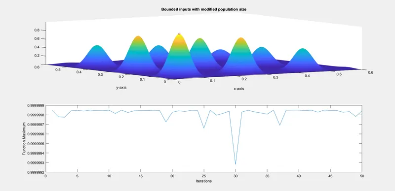
The above result shows that the Bounded inputs with Modified Population size has an accurate solution.
That the maximum point can be found easily, and for this result we used the optimoptions command.
RESULT AND CONCLUSION:
The above results show that the bounded samples with population size have an accurate solution. This is because the code shows the random samples which can start and end at random points.
To overcome the issue, the bounded samples method is used giving the lower and upper limits. (Therefore, it will take the values which are greater than upper Bound or less than the lower bound.)
This loop gives an output with different local maxima with bounded inputs. To conquer this problem, we need to increase the population size as it increases the probability to converge to a global maximum.
The Global maximum of a function can be found by inverting the function. Find the minimum value of the inverted function, the negative of the minimum value will give the global maximum of the function.
Refereces:
Genetic Algorithms - Quick Guide (tutorialspoint.com)
The content for the genetic algorithm syntax, surfc, and other expressions were searched from Help desk in the MATLAB.