Week 5 - Genetic Algorithm

Aim - To optimize the stalagmite function using genetic algorithm techniques using Matlab.

Objective:

Write a code in MATLAB to optimise the stalagmite function and find the global maxima of the function.

Clearly explain the concept of genetic algorithm in your own words and also explain the syntax for ga in MATLAB in your report.

Make sure that your code gives the same output, even if it is made to run several times.

Plot graphs for all 3 studies and for F maximum vs no. of iterations. Title and axes labels are a must, legends could be shown if necessary.

Genetic algorithm:

1. A genetic algorithm (or GA) is a search technique used in computing to find true or approximate solutions to optimization and search problems.
2. (GA)s are categorized as global search heuristics.
3. (GA)s are a particular class of evolutionary algorithms that use techniques inspired by evolutionary biologies such as inheritance, mutation, selection, and crossover (also called recombination).

GA Operators and Parameters:

1. Selection
2. Crossover
3. Mutation.

Selection:

1. The process determines which solutions are to be preserved and allowed to reproduce and which ones deserve to die out. The primary objective of the selection operator is to emphasize the good solutions and eliminate the bad solutions in a population while keeping the population size constant.
2. Functions of the Selection operator, Identify the good solutions in a population Make multiple copies of the good solutions, and Eliminate bad solutions from the population so that multiple copies of good solutions can be placed in the population.

Crossover operator:

1. The most popular crossover selects any two solutions strings randomly from the mating pool and some portion of the strings is exchanged between strings.
2. The selection point is selected randomly.
3. A probability of crossover is also introduced in order to give freedom to an individual solution string to determine whether the solution would go for crossover or not.

Mutation operator:

1. The mutation is the occasional introduction of new features into the solution strings of the population pool to maintain diversity in the population.
2. Though crossover has the main responsibility to search for the optimal solution, the mutation is also used for this purpose.

Procedure:

To solve the global optimization problem we are using the stalagmite mathematical model which is used to develop the local Maxima and Minima, but in our problem we have to get Global Maxima of the function hence we are using the Genetic algorithm here.

Step1:

First, we are defining our search space and creating the one Dimensional arrays x and y with linspace command.

the x and y are input array it does not define the workspace for the genetic algorithm as follows

x = linspace(0,0.6,150);

y = linspace(0,0.6,150);

where:-

0 is an initial value

0.6 is a final value and at last

150 is the number of terms.

Now, creating the two Dimensional array using the meshgrid command as,

[xx,yy]= meshgrid(x,y);

For each value of x and y, we are going to create an input vector (row vector) i.e has two-column.

Note:- the command line [xx, yy]= meshgrid(x,y); is to be used in the separate function name as “get_stalagmite”, which explanation we can get in the “Error and elimination” section further.

we are using the for loop to get the same action multiple times.

for i=1:length(xx)

for j=1:length(yy)

input(1)=xx(i,j);

input(2)=yy(i,j);

f(i,j)= stalagmite(input);

end

end

Where, the stalagmite is a separate function which is based on the formula as follows

Equation Used:

f(x,y)=f1,xf2,xf1,yf2,y

f(x,y)=f1,xf2,xf1,yf2,y

f1.x=[sin(5.1πx+0.5)]6f1.x=[sin(5.1πx+0.5)]6

f1.y=[sin(5.1πy+0.5)]6f1.y=[sin(5.1πy+0.5)]6

f2.x=exp[−4ln(2)(x−0.0667)20.64]f2.x=exp⁡[-4ln⁡(2)(x-0.0667)20.64]

f2.y=exp[−4ln(2)(y−0.0667)20.64]f2.y=exp⁡[-4ln⁡(2)(y-0.0667)20.64]

And now we are writing the final stalagmite Function based on the above formula is as,

function [f] = stalagmite(input_vector)
f1x = (sin((5.1*pi).*input_vector(1)+0.5)).^6;
f1y = (sin((5.1*pi).*input_vector(2)+0.5)).^6;

f2x = exp((((input_vector(1)-0.0667).^2)/0.64).*(-4*log(2)));
f2y = exp((((input_vector(2)-0.0667).^2)/0.64).*(-4*log(2)));
f1=f1x*f1y*f2x*f2y;
f=f1;
end

where the only main point needs to be considered is, the function name and file name should be same.

Step-3:- Syntax Referred for Genetic Algorithm.

In main program we are going to use the one Dimensional arrays x and y with linspace command and as we know the x and y are input array it does not define the workspace for the genetic algorithm.

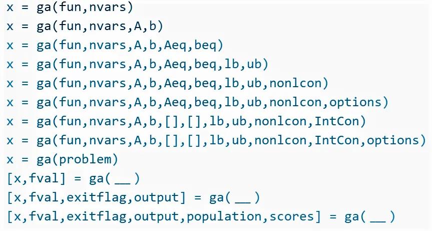
The syntax used for the genetic algorithm is as shown below.

Syntax Referred:

Where:-

x = ga(fun,nvars,A,b) finds a local minimum x to fun, subject to the linear inequalities A*x ≤ b. ga evaluates the matrix product A*x as if x is transposed (A*x').

x = ga(fun,nvars,A,b,Aeq,beq) finds a local minimum x to fun, subject to the linear equalities Aeq*x = beq and A*x ≤ b. (Set A=[] and b=[] if no linear inequalities exist.) ga evaluates the matrix product Aeq*x as if x is transposed (Aeq*x').

x = ga(fun,nvars,A,b,Aeq,beq,lb,ub) defines a set of lower and upper bounds on the design variables, x, so that a solution is found in the range lb ≤ x ≤ ub. (Set Aeq=[] and beq=[] if no linear equalities exist.)

x = ga(fun,nvars,A,b,Aeq,beq,lb,ub,nonlcon) subjects the minimization to the constraints defined in nonlcon. The function nonlcon accepts x and returns vectors C and Ceq, representing the nonlinear inequalities and equalities respectively. ga minimizes the fun such that C(x) ≤ 0 and Ceq(x) = 0. (Set lb=[] and ub=[] if no bounds exist.)

x = ga(fun,nvars,A,b,Aeq,beq,lb,ub,nonlcon,options) minimizes with the default optimization parameters replaced by values in options. (Set nonlcon=[] if no nonlinear constraints exist.) Create options using optimoptions.

x = ga(fun,nvars,A,b,[],[],lb,ub,nonlcon,IntCon) or x = ga(fun,nvars,A,b,[],[],lb,ub,nonlcon,IntCon,options) requires that the variables listed in IntCon take integer values.

Note:- The ga is only used for the minimum function. Hence, to maximize the function we inverse the minimum function.

Matlab Program:

STALAGMITE FUNCTION:

Initially, we will start our code with all the input parameters and define a function into another 'stalagmite(input_vector)'

function [f] = stalagmite_1(input_vector)
x = input_vector(1);
y = input_vector(2);
f1x = (sin((5.1*pi).*input_vector(1)+0.5)).^6;
f1y = (sin((5.1*pi).*input_vector(2)+0.5)).^6;

f2x = exp((((input_vector(1)-0.0667).^2)/0.64).*(-4*log(2)));
f2y = exp((((input_vector(2)-0.0667).^2)/0.64).*(-4*log(2)));
f1=f1x*f1y*f2x*f2y;
f=-f1;
end

Evaluating the stalagmite function:

The code is written to check if the function is returning an output.

The function creates a 3D plot showing the Algorithm.

clear all
close all
clc

%Defining our search space 

x = linspace(0,0.6,150);
y = linspace(0,0.6,150);
n = 50;

%creating a 2D mesh
[xx,yy] = meshgrid(x,y);

%evaluating the stalagmite_1 function
for i=1:length(xx)
    for j =1:length(yy)
        input_vector(1)=xx(i,j);
        input_vector(2)=yy(i,j);
        f(i,j)= stalagmite_1(input_vector);
    end
end
figure(1)
surfc(xx,yy,f)
xlabel('x value')
ylabel('y value')
zlabel('fval')
shading interp
[inputs,fval] = ga(@stalagmite_1,2)

Case-1 (Unbounded Inputs):

For the Unbounded Stalagmites, the code starts with a ‘tic’ having the inputs and optimal function with calling the function.The plot is generated with unbounded stalagmites

tic
for i = 1:n
    [inputs,f_output(i)] = ga(@stalagmite_1,2);
    xopt(i) = inputs(1);
    yopt(i) = inputs(2);
end
study1_time = toc

%plotting of unbounded
figure(2)
subplot(2,1,1)
hold on
surfc(xx,yy,-f)
shading interp
xlabel('x value')
ylabel('y value')
zlabel('fval')
plot3(xopt,yopt,-f_output,'marker','o','markersize',5,'markerfacecolor','r')
title('unbounded inputs')
xlabel('x value')
ylabel('y value')
zlabel('fval')
subplot(2,1,2)
plot(f_output)
xlabel('Iteration')
ylabel('function minimum')

Case-2 (Bounded Inputs):

The code is written for the genetic algorithm function built-in inside MATLAB. An empty array is created with starting and ending points of the x and y values. The plot is created with the inputs in the proper order.

tic
 for i = 1 : n
     [inputs,f_out2(i)] = ga(@stalagmite_1,2,[],[],[],[],[0;0],[1;1]);
     x_out2(i) = inputs(1);
     y_out2(i) = inputs(2);
 end
 study2_time=toc
%plotting of Bounded inputs
 
figure(3)
subplot(2,1,1)
hold on
surfc(x,y,-f)
shading interp
title('Bounded inputs')
xlabel('x values')
ylabel('y values')
zlabel('fval')
plot3(x_out2,y_out2,-f_out2,'marker','o','markersize',6,'markerfacecolor','r')
subplot(2,1,2)
plot(-f_out2)
xlabel('Iterations')
ylabel('Function Maximum')

Case-3 (Bounded Inputs with increased population size):

The code begins with writing ‘optimoptions’.

The plot is then created as the previous method.

tic

options=optimoptions('ga');
options=optimoptions(options,'PopulationSize',500);

for i = 1:n
    [inputs,fopt(i)]= ga(@stalagmite,2,[],[],[],[],[0;0],[1;1],[],[],options);
    xopt(i)=inputs(1);
    yopt(i)=inputs(2);
end

figure(4)

subplot(2,1,1)

hold on

surfc (x,y,-f)
shading interp
plot3(xopt,yopt,-fopt,'marker','o','markersize',5,'markerfacecolor','r')

title('bounded inputs with increases population')
subplot(2,1,2)
plot(-fopt)

xlabel('no. of iterations');
ylabel('function max');

study_time3=toc;​

Main program :

clear all
close all
clc

%Defining our search space 

x = linspace(0,0.6,150);
y = linspace(0,0.6,150);
n = 150;

%creating a 2D mesh
[xx,yy] = meshgrid(x,y);

%evaluating the stalagmite_1 function
for i=1:length(xx)
    for j =1:length(yy)
        input_vector(1)=xx(i,j);
        input_vector(2)=yy(i,j);
        f(i,j)= stalagmite_1(input_vector);
    end
end
figure(1)
surfc(xx,yy,-f)
xlabel('x value')
ylabel('y value')
zlabel('fval')
shading interp
[inputs,fval] = ga(@stalagmite_1,2)

% Study 1: Unbounded statistical Behaviour

tic
for i = 1:n
    [inputs,f_output(i)] = ga(@stalagmite_1,2);
    xopt(i) = inputs(1);
    yopt(i) = inputs(2);
end
study1_time = toc

%plotting of unbounded
figure(2)
subplot(2,1,1)
hold on
surfc(xx,yy,-f)
shading interp
xlabel('x value')
ylabel('y value')
zlabel('fval')
plot3(xopt,yopt,-f_output,'marker','o','markersize',5,'markerfacecolor','r')
title('unbounded inputs')
xlabel('x value')
ylabel('y value')
zlabel('fval')
subplot(2,1,2)
plot(-f_output)
xlabel('Iteration')
ylabel('function minimum')

% Study 2: Statistical Behaviour with lower & upper bounds
tic
 for i = 1 : n
     [inputs,f_out2(i)] = ga(@stalagmite_1,2,[],[],[],[],[0;0],[1;1]);
     x_out2(i) = inputs(1);
     y_out2(i) = inputs(2);
 end
 study2_time=toc
%plotting of Bounded inputs
 
figure(3)
subplot(2,1,1)
hold on
surfc(x,y,-f)
shading interp
title('Bounded inputs')
xlabel('x values')
ylabel('y values')
zlabel('fval')
plot3(x_out2,y_out2,-f_out2,'marker','o','markersize',6,'markerfacecolor','r')
subplot(2,1,2)
plot(-f_out2)
xlabel('Iterations')
ylabel('Function Maximum')


%Study: 3 - Increasing GA Iterations

options=optimoptions('ga')
options=optimoptions(options,'PopulationSize',170)

tic
for i=1:n
[inputs,f_out3(i)]=ga(@stalagmite_1,2,[],[],[],[],[0;0],[0.5;0.5],[],[],options);
x_out3(i)=inputs(1);
y_out3(i)=inputs(2);
end
study3_time = toc
figure(4)
subplot(2,1,1)
hold on
surfc(x,y,-f)
shading interp
title('Increased Iterations')
xlabel('x values')
ylabel('y values')
plot3(x_out3,y_out3,-f_out3,'marker','o','markersize',6,'markerfacecolor','r')
subplot(2,1,2)
plot(-f_out3)
xlabel('Iterations')
ylabel('Function maximum')


saveas(figure(1),'stalagmite_1.jpg')
saveas(figure(2),'Unbounded statistical Behaviour.jpg')
saveas(figure(3),'Statistical Behaviour with lower & upper bounds.jpg')
saveas(figure(4),'Increasing GA Iterations.jpg')

function program:

function [f] = stalagmite_1(input_vector)
x = input_vector(1);
y = input_vector(2);
f1x = (sin((5.1*pi).*input_vector(1)+0.5)).^6;
f1y = (sin((5.1*pi).*input_vector(2)+0.5)).^6;

f2x = exp((((input_vector(1)-0.0667).^2)/0.64).*(-4*log(2)));
f2y = exp((((input_vector(2)-0.0667).^2)/0.64).*(-4*log(2)));
f1=f1x*f1y*f2x*f2y;
f=-f1;
end

Output:

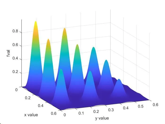
Stalagmite

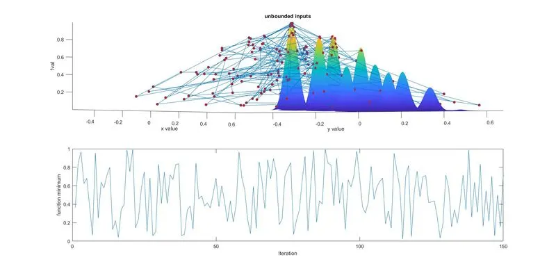
Unbounded statistical Behavior

Hence, Further optimization is required.

Statistical Behavior with lower & upper bounds

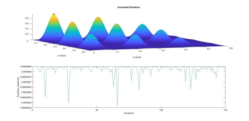
Increasing GA Iterations

Conclusion:

Hence, we are able to optimize the stalagmite function and find the global maxima of the function.

The (ga) is only used for the minimum function therefore to Maximize the function we inversed the minimum function.