Week 5 - Genetic Algorithm

Aim:

To calclulate the gloabAl maxima of a Stalagmite function.

Theory:

Using Genetic Algorithm in matlab we can easily find the global maxima of stalagmite function.

What is stalagmite function?

A family of algorithms known as "genetic algorithms" was invented by Holland and is based on the abstraction of Darwin's theory of the development of biological systems. In the study of adaptive and artificial systems, he was likely the first to employ genetic operators like crossover and recombination, mutation, and selection. In genetic algorithms, there are three main genetic operators or components:

The slalagmite function is given by :

function f = stalagmite(input_vector)

x = input_vector(1);
y = input_vector(2);

f_1x = (sin(5.1.*pi.*x + 0.5))^6;
f_1y = (sin(5.1.*pi.*y + 0.5))^6;

f_2x = exp(-4.*log(2).*((x - 0.0667)^2)/0.64);
f_2y = exp(-4.*log(2).*((y - 0.0667)^2)/0.64);

f = -(f_1x.*f_2x.*f_1y.*f_2y);

end

Case 1:

Calculation of Globbal maxima:

% defining are search space
x = linspace(0,0.6,150);
y = linspace(0,0.6,150);
 
% Iteration Count
num_cases = 500;
 
% Creating a 2D mesh
[xx, yy] = meshgrid(x, y);
 
% Evaluating the stalagmite function
for i = 1:length(xx)
    for j = 1:length(yy)
        input_vector(1) = xx(i,j);
        input_vector(2) = yy(i,j);
        f(i,j) = stalagmite(input_vector);
    end
end
 
for i = 1:num_cases
    [inputs, fval(i)] = ga(@stalagmite,2);
    opt_x(i) = inputs(1);
    opt_y(i) = inputs(2);
end
 
figure(1)
subplot(2,1,1)
surfc(xx,yy,-f)
hold on
 
% Removing gridlines on the 3D surface plot 
shading interp
 
plot3(opt_x,opt_y,-fval,'marker','*','markersize',3)
title('UNBOUNDED INPUTS')
subplot(2,1,2)
plot(-fval)
xlabel('NUMBER OF ITERATIONS')
ylabel('F MAXIMUM')

Case 2:

To study Bounded inputs provided for calculating the value of global maxima.

for i = 1:num_cases
    [inputs, fval(i)] = ga(@stalagmite,2,[],[],[],[],[0;0],[1;1]);
    opt_x(i) = inputs(1);
    opt_y(i) = inputs(2);
end
 
figure(2)
subplot(2,1,1)
surfc(xx,yy,-f)
xlabel('x value')
ylabel('y value')
hold on
shading interp
plot3(opt_x,opt_y,-fval,'marker','*','markersize',3)
title('BOUNDED INPUTS')
subplot(2,1,2)
plot(-fval)
xlabel('NUMBER OF ITERATIONS')
ylabel('F MAXIMUM')

Case 3:

The thrid input provides bounded inputs with varied population size for getting better values of Global maxima.

options = optimoptions('ga');
options = optimoptions(options,'PopulationSize',600);
for i = 1:num_cases
    [inputs, fval(i)] = ga(@stalagmite,2,[],[],[],[],[0;0],[1;1],[],[],options)
    opt_x(i) = inputs(1);
    opt_y(i) = inputs(2);
end
 
figure(3)
subplot(2,1,1)
surfc(xx,yy,-f)
xlabel('x value')
ylabel('y value')
hold on
shading interp
plot3(opt_x,opt_y,-fval,'marker','*','markersize',3)
title('BOUNDED INPUTS WITH ALTERED POPULATION SIZE')
subplot(2,1,2)
plot(-fval)
xlabel('NUMBER OF ITERATIONS')
ylabel('F MAXIMUM')

Explanation of the code:

• First thing is to mention the stalagmite function with appropriate argument vectors.
• The program has been divided three studies based on the previous.
• First study explain the unbounded inputs.
• Second case deals with the bounded inputs providing a better way for limitations previously faced.
• Third study gives optimised result of the two cases.
• The final step is plotting the results which gives the complete idea of the code.

Results:

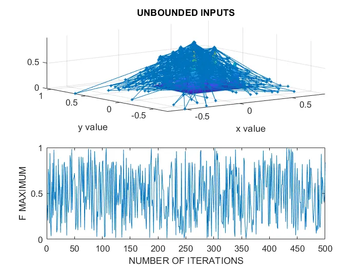
The results in the girst case varies with large interval providing a good idea for the study of maxima.But we can see that the value of Global maxima lies from o to 1 so we have to go for another step for calculating the value of global maxima.

Study 2:

From the above obtained plot we can get to know that the value of good maxima lies somewhere between [0.9 to 1].To get better unterstanding we can specify a population size taht can justify our output and provides us with a close solution.`

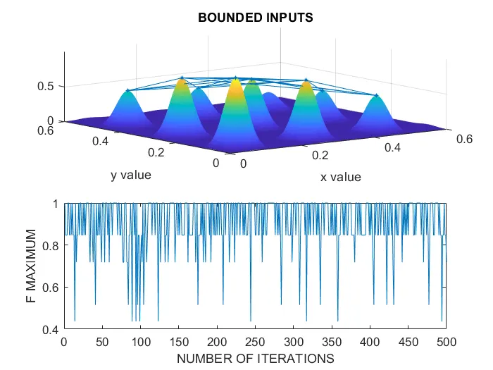
Result:We can observe that by the use of 'Population Method'within the bounded input the probability of determining the exact value of the Global Maxima increases in a substantial way.Now the assumed value of populaion size is '600'.

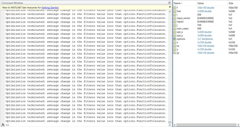
The value of global maxima comes out to be 0.9999985

Conclusion:

The global maxima is calculated using the Population sizing and plots are showing the visual representaions of our calculations.