Project 2 - Rankine cycle Simulator
Rankie cycle simulator:
Aim:
Creation of Rankine cycle simulator from given input and reading the data from standard thermodynamic library of steam table.
Objective:
- To create a Rankine Cycle simulator in MATLAB.
- To calculate the state point using function XSteam.
- To plot the T-S and H-S curve for given input in Rankine Cycle.
- To get output in the command window for each state point in cycle.
Description:
The Rankine cycle is an idealized thermodynamic cycle describing the process by which certain heat engines, such as steam turbines or reciprocating steam engines, allow mechanical work to be extracted from a fluid as it moves between a heat source and heat sink. The Rankine cycle is named after William John Macquorn Rankine, a Scottish polymath professor at Glasgow University.
Heat energy is supplied to the system via a boiler where the working fluid (typically water) is converted to a high pressure gaseous state (steam) in order to turn a turbine. After passing over the turbine the fluid is allowed to condense back into a liquid state as waste heat energy is rejected before being returned to boiler, completing the cycle. Friction losses throughout the system are often neglected for the purpose of simplifying calculations as such losses are usually much less significant than thermodynamic losses, especially in larger systems.
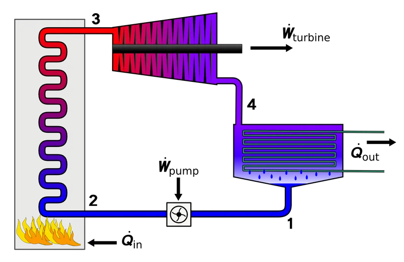
The components in the rankie cycle are as follows:
a) Turbine (1-2)
b)Condenser (2-3)
c)Pump(3-4)
d)Boiler(4)
The rankie cycle consists of four processes namely:
Process 1-2: Isentropic Expansion: The superheated vapor is expanded isentropically in the turbine, thus producing work which may be converted to electricity. The exit condition of turbine may exits in 3 states i.e, superheated state, saturated vapor state or liquid-vapor mix state.Here the tempreature and pressure of the vapour is reduced and can result in some condensation.
Process 2-3: Isobaric Heat Rejection: The vapor-liquid mixture leaving the turbine is condensed at constant low pressure, usually in a surface condenser using cooling water. In well designed and maintained condensers, the pressure of the vapor is well below atmospheric pressure, approaching the saturation pressure of the operating fluid at the cooling water temperature.
Process 3-4: Isentropic Compression. The pressure of the condensate is raised isentropically in the feed pump. Because of the low specific volume of liquids, the pump work is relatively small and often neglected in thermodynamic calculations.
Process 4-1: Isobaric Heat Transfer: High pressure liquid enters the boiler from the feed pump and is heated to the saturation temperature. Further addition of energy causes evaporation of the liquid until it is fully converted to saturated steam. Further addition of energy takes the saturated steam into superheated state.
Q.Heat flow rate to or from the system
m.Mass flow rate
W.Mechanical power consumed by or provided to the system.
 .Thermodynamic efficiency of the process
 .Icentropic efficiency of compression and expansion.
 .Entalpies at indicated points in T.s diagram
 .Final Specific Enthalpy
 .Pressure before and after the compression process.
In general, the efficiency of a simple rankine cycle can be written as

Each of the next four equations is derived from the energy and mass balance for a control volume. defines the thermodynamic efficiency of the cycle as the ratio of net power output to heat input. As the work required by the pump is often around 1% of the turbine work output, it can be simplified.




When dealing with the efficiencies of the turbines and pumps, an adjustment to the work terms must be made:


Writing the code
fprintf(' Rankine Cycle\n ')
fprintf('1-2 is Isentropic Expansion in Turbine\n')
fprintf(' 2-3 is constant pressure heat removal\n')
fprintf(' 3-4 is Isentropic Compression in Pump \n')
fprintf(' 4-1 Constant pressure Heat addition in Boiler\n')
Rankine Cycle
1-2 is Isentropic Expansion in Turbine
2-3 is constant pressure heat removal
3-4 is Isentropic Compression in Pump
4-1 Constant pressure Heat addition in Boiler

% Entering the input data for calculation of state points
p1 = 50; %Pressure at Turbine Inlet
T1 = 500; %Temperature at Turbine Inlet
p2 = 5; %Pressure at Condenser

% Entering the input data to calculate the state points
p1 = 50; %Pressure at Turbine Inlet
T1 = 500; %Temperature at Turbine Inlet
p2 = 5; %Condenser Pressure


% For state 1 taking data from the xsteam file
h1 = XSteam('h_pT', p1, T1); % Enthaply at pressure and Temp 1
s1 = XSteam('s_pT', p1, T1); % Entropy at pressure and Temp 1


% For state point 2 taking data from Xsteam file
s2 = s1; % Isentropic Expansion
sf2 = XSteam('sL_p', p2); % Saturated liquid entropy at pressure 2
sg2 = XSteam('sV_p', p2); % Saturated vapour entropy at pressure 2
x2 = (s2-sf2)/(sg2-sf2); % Vapour Fraction at state point 2
hf2 = XSteam('hL_p', p2); % Saturated liquid Enthalpy at pressure 2
hg2 = XSteam('hV_p', p2); % Saturated vapour Enthalpy at pressure 2
h2 = hf2 + (x2*(hg2-hf2)); % Enthalpy at state point 2


% For state point 3 taking data from Xsteam file for
p3 = p2; % Constant Pressure heat rejection process
s3 = XSteam('sL_p', p3); % Saturated liquid entropy at Pressure 3
h3 = XSteam('hL_p', p3); % Saturated liquid Enthalpy at Pressure 3


% For state point 4 taking data from Xsteam file
s4 = s3; % Isentropic Compression process
p4 = p1; % Constant Pressure heat rejection


% Work done in Turbine for the rankine cycle
W_T = h1-h2; %Ethalpy at state point 1- Enthalpy at state point 2

% Work done required for pump
v3 = XSteam('vL_p',p3); % Saturated Liquid Vapour at pressure 3
W_P = v3*(p4-p3)*100; % Work done for pump
h4 = h3 - W_P; % Enthalpy at State point 4


% Net work done for Rankine Cycle
W_net = W_T - W_P;


% Heat Addition to System
Q_in = h1-h4;


% Heat Rejection from System
Q_out = h2-h3;


% Thermal Efficiency of Rankine Cycle
T_eff = (W_net/Q_in)*100;


%specific steam consumption = (Mass flow rate / Net work done)
Sp_S = (3600/W_net);


% Calculation of Temperature at All state Point 2, 3 and 4
T3 = XSteam('Tsat_p',p3); % Saturation Temperature at Pressure 3
T2 = T3; % Due to Constant Pressure Heat addition
Cp4 = XSteam('Cp_ps',p4,s4); % Specific isobaric heat capacity
Cv4 = XSteam('Cv_ps',p4,s4); % Specific isochoric heat capacity
k = Cp4/Cv4;
T4 = T3/((p3/p4)^((k-1)/k)); % Temperature at State point 4

% Calculation of Other constant for saturated liquid and Vapour
T6 = XSteam('Tsat_p', p1); % Saturated Temperature at Pressure 1
s5 = XSteam('sL_p', p1); % Saturated Liquid entropy at pressure 1
s6 = XSteam('sV_p', p1); % Saturated Vapour entropy at Pressure 1
h5 = XSteam('hL_p', p1); % Saturated Liquid Enthalpy at Pressure 1
h6 = XSteam('hV_p', p1); % Saturated Vapour Enthalpy at pressure 1
T5 = T6;


%Plotting for Saturation Line
T = linspace(1,560,1000);
for i = 1:length(T)
sf(i) = XSteam('sL_T' ,T(i)); % Saturated Liquid Entropy
sg(i) = XSteam('sV_T' ,T(i)); % Saturated Vapour Entropy
hf(i) = XSteam('hL_T' ,T(i)); % Saturated Liquid Enthalpy
hg(i) = XSteam('hV_T' ,T(i)); % Saturated Vapour Enthalpy

end
% Plotting T-S Diagram for Rankine Cycle
figure(1)
hold on
plot(sf,T,'color','b','linewidth',2)
plot(sg,T,'color','b','linewidth',2)
plot([s1 s2],[T1 T2], 'color', 'r', 'linewidth',3)
plot([s2 s3],[T2 T3], 'color', 'r', 'linewidth',3)
plot([s3 s4],[T3 T4], 'color', 'r', 'linewidth',3)
plot([s4 s5],[T4 T5], 'color', 'r', 'linewidth',3)
plot([s5 s6],[T5 T6], 'color', 'r', 'linewidth',3)
s_1 = linspace(s6,s1,1000);
for j = 1:length(s_1)
Tc(j) = XSteam('T_ps',p1,s_1(j));


end
plot(s_1,Tc,'color','r','linewidth',3)
text(s1+0.1, T1, '1')
text(s2+0.1, T2, '2')
text(s3, T3-20, '3')
text(s4, T4+20, '4')
title('Temperature Vs Entropy')
xlabel('Entropy (Kj/kg-k)')
ylabel('Temeperature (Deg. Celcius)')
legend('Saturation Curve')
figure(1)
figure(2)
hold on
plot(sf,T,'color','b','linewidth',2)
plot(sg,T,'color','b','linewidth',2)
plot([s1 s2],[T1 T2], 'color', 'r', 'linewidth',3)
plot([s2 s3],[T2 T3], 'color', 'r', 'linewidth',3)
plot([s3 s4],[T3 T4], 'color', 'r', 'linewidth',3)
plot([s4 s5],[T4 T5], 'color', 'r', 'linewidth',3)
plot([s5 s6],[T5 T6], 'color', 'r', 'linewidth',3)
s_1 = linspace(s6,s1,1000);
for j = 1:length(s_1)
Tc(j) = XSteam('T_ps',p1,s_1(j));
delete(figure(2))

% Plotting H-S Diagram for Rankine Cycle
figure(3)
hold on
plot(sf,hf,'color','b','linewidth',2)
plot(sg,hg,'color','b','linewidth',2)
plot([s1 s2],[h1 h2],'color','r','linewidth',3)
plot([s2 s3],[h2 h3],'color','r','linewidth',3)
plot([s3 s4],[h3 h4],'color','r','linewidth',3)
hc = linspace(h4,h5,100);
for k = 1:length(hc)
s_c(k) = XSteam('s_ph',p1,hc(k));
end
plot(s_c,hc,'color','r','linewidth',3)
plot([s5 s6],[h5 h6],'color','r','linewidth',3)
for l = 1:length(s_1)
h_c(l) = XSteam('h_ps',p1,s_1(l));


end
plot(s_1,h_c,'color','r','linewidth',3)
text(s1+0.1,h1,'1')
text(s2+0.1,h2,'2')
text(s3,h3-100,'3')
text(s4,h4+200,'4')
title('Enthalpy Vs Entropy')
xlabel('Entropy (Kj/kg-k)')
ylabel('Enthalpy (KJ/Kg)')
legend('Saturation Curve')

end
plot(s_1,h_c,'color','r','linewidth',3)
text(s1+0.1,h1,'1')
text(s2+0.1,h2,'2')
text(s3,h3-100,'3')
text(s4,h4+200,'4')
title('Enthalpy Vs Entropy')
xlabel('Entropy (Kj/kg-k)')
ylabel('Enthalpy (KJ/Kg)')
legend('Saturation Curve')


% Displaying Results in Command window
disp('Results of Rankine Cycle')
fprintf('At state point 1\t\t\t\t\t')
fprintf('At state Point 2\n')
fprintf('P1 = %10f in Bar\t\t\t\t',p1);
fprintf('P2 = %10f in Bar\n',p2);
fprintf('T1 = %11f in Deg.Celcius\t\t',T1);
fprintf('T2 = %11f in Deg.Celcius\n',T2);
fprintf('H1 = %12f in KJ/Kg\t\t\t',h1);
fprintf('H2 = %12f in KJ/Kg\n',h2);
fprintf('S1 = %9f in KJ/Kg-k\t\t\t',s1);
fprintf('S2 = %9f in KJ/Kg-k\n',s2);
fprintf('\n')
fprintf('At state point 3\t\t\t\t\t')
fprintf('At state Point 4\n')
fprintf('P3 = %10f in Bar\t\t\t\t',p3);
fprintf('P4 = %10f in Bar\n',p4);
fprintf('T3 = %11f in Deg.Celcius\t\t',T3);
fprintf('T4 = %11f in Deg.Celcius\n',T4);
fprintf('H3 = %12f in KJ/Kg\t\t\t',h3);
fprintf('H4 = %12f in KJ/Kg\n',h4);
fprintf('S3 = %9f in KJ/Kg-k\t\t\t',s3);
fprintf('S4 = %9f in KJ/Kg-k\n',s4);
fprintf('\n')
fprintf('Turbine Work Done = %14f in KJ/Kg\n',W_T)
fprintf('Pump Work Done = %15f in KJ/Kg\n',W_P)
fprintf('Net Work Done = %17f in KJ/Kg\n',W_net)
fprintf('Thermal Efficiency = %13f in percent\n',T_eff)
fprintf('Sp. Steam Consumption = %f in KJ/Kw\n',Sp_S)
Explanation of the plots:
We are changing some value in the inputs by increasing the inlet pressure and temperature along with condenser pressure also which results in following graphs.
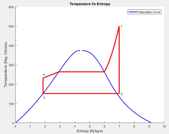
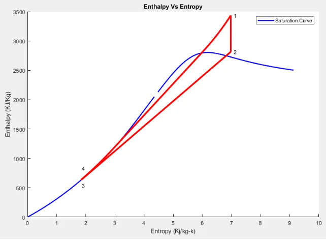
Inlet value for tempreature and pressure is as
Inlet Pressure for turbine =30bar
Inlet tempreature for turbine=400deg.cel
Pressure in condenser=0.05bar
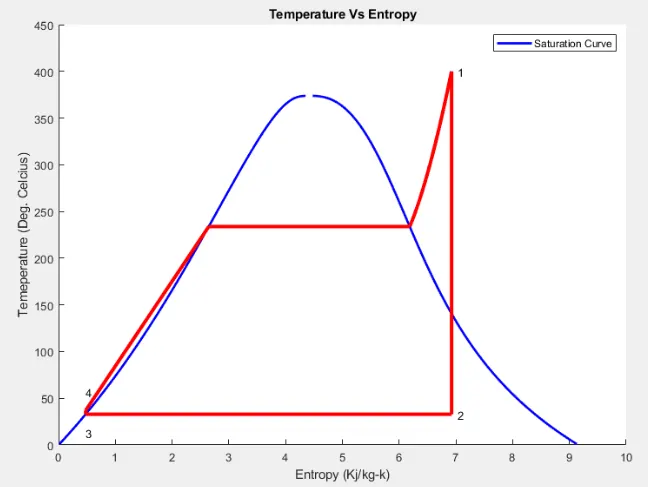
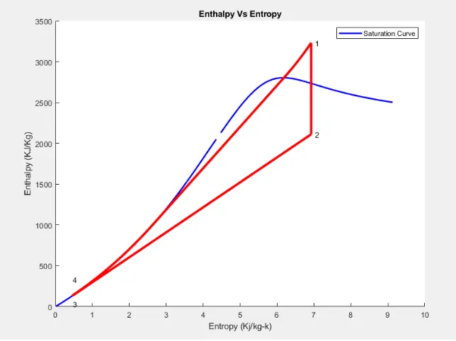
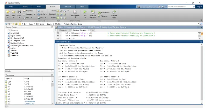
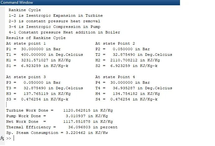
Above graph shows that the turbine work done is approx 1120 kj/kg ,Pump work and net work as 3.01kj/kg and 1117.85K j/kg and thermal efficiency is 36.09.
We can clearly see that by increasing the tempreature and the pressure in the turbine, the efficiency of the cycle gets reduced.
Conclusion:
We have successfully plotted the Rankie cycle diagram by using the xsteam tabel and the inputs given to us.