Week 5 - Genetic Algorithm

AIM

Genetic Algorithm

Objective

To Write a code in MATLAB to optimise the stalagmite function and find the global maxima of the function.

Software Used

Matlab R2021a

Introduction

MATLAB^® combines a desktop environment tuned for iterative analysis and design processes with a programming language that expresses matrix and array mathematics directly. It includes the Live Editor for creating scripts that combine code, output, and formatted text in an executable notebook.

A genetic algorithm is a natural process that is used for the selection of the fittest individuals. The main use of the genetic algorithm is for reproduction to produce offspring of the next generation, this process of selecting and reproducing the fittest individual is inspired by Charles Darwin’s and named it the "Theory of evolution".

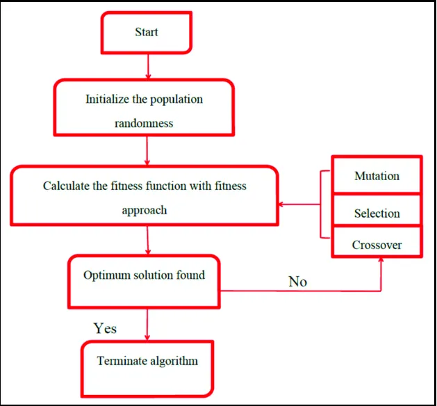
The five phases of GA are:

Initial population
Fitness function
Selection
Crossover
Mutation

Advantages of GAs

• GAs have various advantages that have made them immensely popular. These include −
• Does not require any derivative information (which may not be available for many real-world problems).
• Has very good parallel capabilities.
• Optimizes both continuous and discrete functions and also multi-objective problems.
• Provides a list of “good” solutions and not just a single solution.
• Useful when the search space is very large and there are a large number of parameters involved.
• Always provide good results over time.

Limitations of GAs

• If not implemented properly, the GA may not converge to the optimal solution.
• Where there is simple problem and for that the derivative values is known then this is not suited i.e genetic algorithm

Stalagmite function

Stalagmite is a type of rock formation that rises from the floor of a cave due to the accumulation of material deposited on the floor from ceiling drippings. Stalagmite function is the mathematical function which generates similar shapes to stalagmites.

INPUT CODE

• FUNCTION CODE

function[inputs] = stalagmite(input_vector)
x1 = input_vector(1);
y1 = input_vector(2);

f1_x = (sin(5.1*pi*x1+0.5))^6;
f1_y = (sin(5.1*pi*y1+0.5))^6;

f2_x = exp(-4*log(2)*(x1-0.0667)^2/0.64);
f2_y = exp(-4*log(2)*(y1-0.0667)^2/0.64);

[inputs] = -(f1_x*f1_y*f2_x*f2_y);
end

• MAIN CODE

close all
clear all
clc

% Defining search space
x = linspace(0,0.6,150);
y = linspace(0,0.6,150);
[xx yy] = meshgrid(x,y);

% Evaluating stalagmite function
for i = 1:length(xx)
    for j = 1:length(yy)
        input_vector(1) = xx(i,j);
        input_vector(2) = yy(i,j);
        f(i,j) = stalagmite(input_vector);
    end
end

% Ploting Stalagmite Function
surfc(xx,yy,f)
xlabel('x axis')
ylabel('y axix')
shading interp
[inputs,fval] = ga(@stalagmite,2);
title('Stalagmite function')

num_cases = 50;

% Study 1 - Statistical behaviour
tic
for i = 1:num_cases
    [inputs,fopt(i)] = ga(@stalagmite,2);
    xopt(i) = inputs(1);
    yopt(i) = inputs(2);
end
study_time1 = toc

% Plotting Study 1
figure(1)
subplot(2,1,1)
hold on
surfc(x, y, f)
shading interp
plot3(xopt,yopt,fopt,'marker','o','markersize',5,'markerfacecolor','r')
title('Unbounded Inputs')
subplot(2,1,2)
plot(fopt)
xlabel('Iterations')
ylabel('Function Maximum')

% Study 2 - With upper and lower bounds
tic
for i = 1:num_cases
    [inputs,fopt(i)] = ga(@stalagmite,2,[],[],[],[],[0,0],[1,1]);
    xopt(i) = inputs(1);
    yopt(i) = inputs(2);
end
study_time2 = toc

% Plotting Sudy 2
figure(2)
subplot(2,1,1)
hold on
surfc(x, y, f)
shading interp
plot3(xopt,yopt,fopt,'marker','o','markersize',5,'markerfacecolor','r')
title('Bounded Inputs')
subplot(2,1,2)
plot(fopt)
xlabel('Iterations')
ylabel('Function Maximum')

% Study 3 - Increasing GA iterations

options = optimoptions('ga');
options = optimoptions(options,'PopulationSize',500)

tic
for i = 1:num_cases
    [inputs,fopt(i)] = ga(@stalagmite,2,[],[],[],[],[0,0],[1,1],[],[],options);
    xopt(i) = inputs(1);
    yopt(i) = inputs(2);
end
study_time3 = toc

% Plotting Study 3
figure(3)
subplot(2,1,1)
hold on
surfc(x, y, f)
shading interp
plot3(xopt,yopt,fopt,'marker','o','markersize',5,'markerfacecolor','r')
title('Bounded With Increased Population')
subplot(2,1,2)
plot(fopt)
xlabel('Iterations')
ylabel('Function Maximum')

OUTPUT

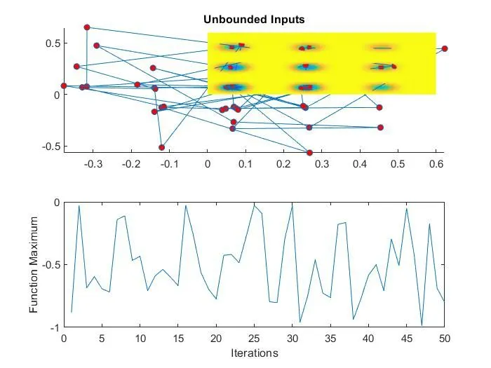
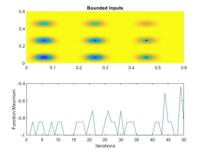
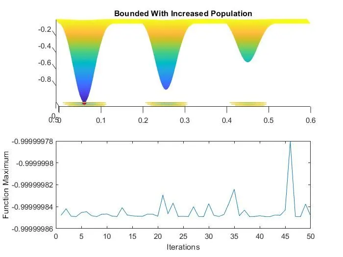
With the increased population size we get the most accurate result which is in between 0.99999981 to 0.99999984.

CONCLUSION

The code have been execute successfully