Week 5 - Genetic Algorithm

Aim: To optimize the Stalagmite function and obtain the Global maximum for the stalagmite function using the Genetic Algorithm and explain the various ways of approach with there significance.

Objective of the project:

1. Specify the area of Stalagmite function.
2. Code the function for the Stalagmite.
3. Plot the surf for the Stalagmite output.
4. Now using the Genetic Algorithm find the optimized Global maximum for the Stalagmite output.
5. Here three cases are taken to obtain the Global maximum for the function output:
   1. Unbounded (No upper and lower bounds are defined).
   2. Bounded (Upper and lower bounds are defined for the GA).
   3. Bounded with modified Population size (Along with upper and lower bound the population size is altered).
6. The results are plotted and the significance and draw backs of the case are studied.
7. Stopping criteria, significance of running multiple iterations are explained.

1. Code-Genetic Algorithm:

   1. close all     % Closing all the open graphs tabs
      clear all     % Clearing all the garbafge values
      clc           % Clearing the command tab
      
      
      % Defining the inputs to the meshgrid generation
      x = linspace(0,0.6,150);
      y = linspace(0,0.6,150);
      
      % Creating a 2D mesh
      [xx,yy] = meshgrid(x,y);
      
      % Evaluating the stalagmite function
      for i = 1:length(xx);
          for j = 1:length(yy);
              input_vector(1) = xx(i,j); % Assigning the grid x and y values to variables
              input_vector(2) = yy(i,j);
              f(i,j) = stalagmite_fun2(input_vector);  % Calling the stalagmite function
          end        % Closing second for loop
      end            % Closing first for loop
      
      % Actual plot output of the stalagmite function:
      figure(1)
      surfc(xx,yy,-f)
      xlabel('x-axis')
      ylabel('y-axis')
      zlabel('Stalagmite output')
      title('Actual')
      shading interp % Clearing the shaded lines on the surf plots 
      
      % Creating the surf plot for the meshgrid(as x,y) and stalagmite(as z)
      
      figure(2)
      surfc(xx,yy,f)
      xlabel('x-axis')
      ylabel('y-axis')
      zlabel('Stalagmite output')
      title('Inverted')
      % Clearing the shaded lines on the surf plots 
      shading interp
      
      % Case-1: Unbounded (Here the Genetic Algorithum picks random values even from out side of the study region) 
      
      num_case = 50;      % To run the case for 50 times
      tic                 % calculte the time taken by this part to complete the operations
      for j = 1:num_case  % For loop for 50 times.
          [inputs_u,fopt(j)] = ga(@stalagmite_fun2,2);
          xt(j) = inputs_u(1);
          yt(j) = inputs_u(2);
          
      end
      study_time_unbounded = toc
      
      %  Plotting
      figure(3)
      
      subplot(2,1,1)            % Using subplot for better comparsion of values for  
      surf(xx,yy,-f)
      hold on
      shading interp            % To clear the lines from the surf plot
      plot3(xt,yt,-fopt,'marker','o','markersize',5)  
      xlabel('X-values_u')         % Labeling the x, y and z axis
      ylabel('Y-values_u')
      zlabel('Stalagmite output')
      title('Unbounded case')
      
      subplot(2,1,2)           
      plot(-fopt)
      xlabel('Iterations_u')
      ylabel('Maximum values_u')
      
      
      % Case-2 Bounded (Here the upper and lower bounds of the search area for
      % randomization are prescribed)
      
      % Running the ga for 50 times
      tic
      for k = 1:num_case
          [inputs_b, fopt_b(k)] = ga(@stalagmite_fun2,2,[],[],[],[],[0;0],[0.6;0.6]); % Defining the bounds
          xb(k) = inputs_b(1);
          yb(k) = inputs_b(2);
          
      end
      study_time_bounded = toc
      % Plotting
      figure(4)
      
      subplot(2,1,1)
      surf(xx,yy,-f)
      hold on
      shading interp
      plot3(xb,yb,-fopt_b,'marker','o','markersize',5)
      xlabel('X-values_b')         % Labeling the x, y and z axis
      ylabel('Y-values_b')
      zlabel('Stalagmite output')
      title('Bounded case')
      
      subplot(2,1,2)
      plot(-fopt_b)
      xlabel('Iterations_b')
      ylabel('Maximum values_b')
      
      
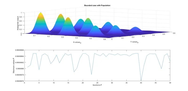
      % Case-3 Bounded and specified population size(here along with the upper
      % and lower bounds the population size is defined)
      
      options = optimoptions('ga'); % Defining ga inbuilt function need to be modified 
      options = optimoptions(options, 'Populationsize', 270); % Indicating that Poulation size needs to be altered, Modifing the population size to 270
      
      % Running the ga for 50 times
      
      tic
      for l = 1: num_case
          [inputs_P, fopt_P(l)] = ga(@stalagmite_fun2,2, [],[],[],[],[0;0],[0.6;0.6],[],[], options); % Calling the changed options settings for this particular case
          xp(l) = inputs_P(1);
          yp(l) = inputs_P(2);
          
      end
      study_time_bounded_population = toc
      % Plotting 
      figure(5)
      subplot(2,1,1)
      surf(xx,yy,-f)
      hold on
      shading interp
      plot3(xp,yp,-fopt_P,'marker','o','markersize',5)
      xlabel('X-values_P')         % Labeling the x, y and z axis
      ylabel('Y-values_P')
      zlabel('Stalagmite output')
      title('Bounded case with Population')
      
      subplot(2,1,2)
      plot(-fopt_P)
      xlabel('Iterations-P')
      ylabel('Maximum values-P')
      
      
      
           
      
          
      
      
      

2. Code-Stalagmite function:

   1. 
      %staligmite function
      
      function [f] = stalagmite_fun2(input_vector)  % Defining the name of the function
      
          x = input_vector(1); % Assing the input_vector values to variable as x and y (unpacking)  
          y = input_vector(2);
      
          f1x = (((sin(5.1*pi*x + 0.5)))^6);   % Calculating the individual part
      
          f1y = ((sin(5.1*pi*y + 0.5))^6);
      
          f2x = (exp(((-2.77259)*(x-0.0667)^2)/(0.64)));
      
          f2y = (exp(((-2.77259)*(y-0.0667)^2)/(0.64)));
      
          [f] = -(f1x*f1y*f2x*f2y); % Here the stalagmite function is multiplied by negative sign 
                                    % to inverse the stalagmite output in the z-axis, as GA only optimizes for the  global minima
      
      end        % End of the function definition
      
      
      
      

Results and discussion:

1. Output of the stalagmite function (Actual and Inverted):
   
   1. 
   2. 
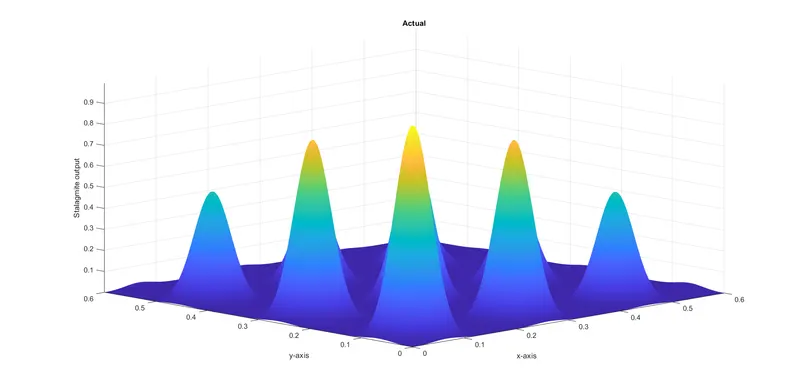
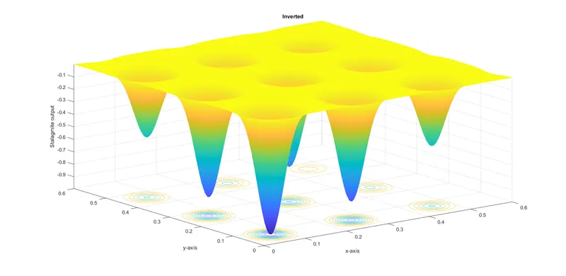
   3. Used to find the global minima by using the genetic algorithm.
2. Case-1 Unbounded Optimized output:
   1. 
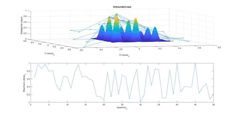
   2. Here in this case the algorithm choses random population without any boundaries resulting in more dispersed output.
   3. Here the optimized values are ranging from 0-1 which is not at all accurate.
   4. This case types cannot be used for this kind of function/problems.
   5. Here the algorithm is run for 50 times.
3. Case-2 Bounded Optimized output:
   1. 
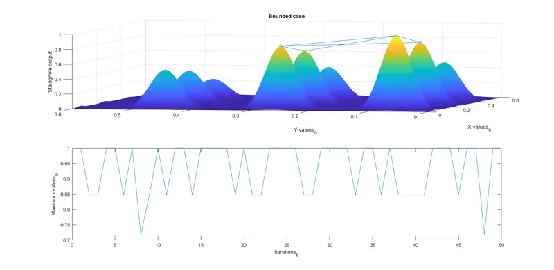
   2. Here the algorithm selects the population in the region defined in the upper and lower bounds.
   3. Here the output/optimized results are more confined and near to the optmized value compared to case-1.
   4. It can be seen that the optimized values are much closer to the actual maximum value (0.7 - 1) compared to case-1 (subplot - 2).
   5. Here the algorithm is run for 50 times.
4. Case-3 Bounded with population modification Optimized output:
   1.