Week 5 - Genetic Algorithm
AIM: To write code to calculate Global Maxima using Genetic Algorithm, using MATLAB .
PROCEDURE:
The satalagmite function is defined separately . This function is later called into the main GA program .
Now we define the x and y inputs using linspace command .
Then the input vectors are transformed into array[X,Y], so that it can be used to evalute function of two variables and plot three dimension mesh/surface plots.
Now the values in the different matrixs created can be put as an input into the function that we have created by calling it. By this we can get the stalagmite function at various values of x and y .
Now since we have got the value of the function at various values we now need to calculate the maxima value , which can be calculated using the ga command , which is an in-built function in MATLAB.
Then, the total number of time the ga needs to run is defined using num_cases, and with help of for loop ga is made to run for each iteration and the value is stored in an array.
GA generaally gives the minima value ,but we need the maxima hence we can just inverse the stalagmite function by introducing a 'Negative sign' .
The total study time is calculted using the 'tic' and 'toc' connand at the start and end of the ga for loop respectively.
The results are then plotted using the surfc command and plot command.
GA is made to run for 3 iterations, weith each iteration having bounded inputs, unbounded inputs and increasing population size.
The stalagmite function is as follows:
The above function is defined in the stalagmite function in MATLAB as shown below.
function f = stalagmite(input_vector)
x= input_vector(1);
y= input_vector(2);
f1_x= (sin(5.1*pi*x+0.5))^6;
f2_y= (sin(5.1*pi*y+0.5))^6;
f3_x= exp(-4*log(2)*(x-0.067)^2/0.64);
f4_y= exp(-4*log(2)*(y-0.067)^2/0.64);
f=-(f1_x*f2_y*f3_x*f4_y);
end
The format for writing genetic algorithum in MATLAB is as follows:
x=ga(fun,nvars,A,b,Aeq,beq,lb,ub,nonlcon,options)
1.x is the local minima point .
2. fun is the function to be called
3. A and b are used to of indicate any kind inequalities bthat exist in the function .
4. Aeq and beq also denotes the inequalities .
5. nvars indicates the no of variables used.
6. lb = lower bound .
7. ub = upper bound .
8. nonlcon gives a two vectors representing inequalities and equalities.
9. option is used to preform assitional operation like increasing population size . This is done with the help of "optimoptions".
1st iteration:
IN the first iteration, the behaviour of the algorithm is studied by not defining the limits. The GA does not run within a particular search space , since we have not defined bounds.
clear all
close all
clc


x= linspace(0,0.6,150);% X value inputs
y= linspace(0,0.6,150);% Y value inputs
% Even though search space is defined GA algorithm donot run within this searchspace
[X,Y]= meshgrid(x,y);

num_cases=50;% GA runs for 50 iterations


for  i=1:length(X)
for    j=1:length(Y)
input_vector(1)=X(i,j);
input_vector(2)=Y(i,j);
f(i,j)=stalagmite(input_vector);
end
end
tic % study time count start
for i=1:num_cases
    [inputs,f_opt(i)]= ga(@stalagmite,2);% GA function is used to run the stalagmite data and give the optimal solutions.
    x_opt(i)= inputs(1);
    y_opt(i)= inputs(2);
    opt_f(i)=-f_opt(i);%GA gives us Minima value . Inverse f_opt is tajen for Maxima value.
end
study1_time = toc; % study time count end

subplot(2,1,1)
hold on

surfc(X,Y,-f); % Generation of satlagmite funtion .

shading interp % To bring visually smooth curve surface without mesh lines
plot3(x_opt,y_opt,-f_opt,'marker','o','markersize',4,'markerfacecolor','r')% plotting the optimum values with a red dot marker along the stalagmite 3D curves
title('Unbounded inputs')
subplot(2,1,2)
plot(-f_opt)% plot of opt_f for every iteratons
xlabel('Number of iteration')
ylabel('Function Max')
2nd iteration :
Here the lower and upper bounds are defined so as to know the boundaries within which the global maxima lies . In other words we are defining a definite space within which the global maxima is to be found.
clear all
close all
clc


x= linspace(0,0.6,150);% X value inputs
y= linspace(0,0.6,150);% Y value inputs
% Even though search space is defined GA algorithm donot run within this searchspace
[X,Y]= meshgrid(x,y);

num_cases=100; % GA runs for 100 iterations


for  i=1:length(X)
for    j=1:length(Y);
input_vector(1)=X(i,j);
input_vector(2)=Y(i,j);
f(i,j)=stalagmite(input_vector);% stalagmite function is called for every loop and output is stored in f.
end
end
tic % study time count start
for i=1:num_cases;
% objective function is stalagmite and the number of veriable is 2.
% A,B, Aeq and Beq = [] as there is no linear equaalities and inequalities constraints in this function
% lower boundary of varaibles x and y in ga alogorithmn is set as [0,0]
% upper boundary of varaibles x and y in ga alogorithmn is set as [0.6,0.6]
    [inputs,f_opt(i)]= ga(@stalagmite,2,[],[],[],[],[0,0],[0.6,0.6]);% GA function is used to run the stalagmite data and give the optimal solutions.
    x_opt(i)= inputs(1);
    y_opt(i)= inputs(2);
    opt_f(i)=-f_opt(i)%GA gives us Minima value . Inverse f_opt is tajen for Maxima value.
end
study1_time = toc  % study time count end

subplot(2,1,1)
hold on
surfc(X,Y,-f) % Generation of satlagmite funtion
shading interp % To bring visually smooth curve surface without mesh lines
plot3(x_opt,y_opt,-f_opt,'marker','o','markersize',4,'markerfacecolor','r')% plotting the optimum values with a red dot marker along the stalagmite 3D curves
title('with bounded inputs')
subplot(2,1,2)
plot(-f_opt) % plot of opt_f for every iteratons
xlabel('Number of iteration')
ylabel('Function Max')
3rd iteraation:
In this iteration the population size is increased so as to converge to the global maxima .
clear all
close all
clc


x= linspace(0,0.6,150);
y= linspace(0,0.6,150);
[X,Y]= meshgrid(x,y);

num_cases=150;% GA runs for 150 iterations


for  i=1:length(X)
for    j=1:length(Y);
input_vector(1)=X(i,j);
input_vector(2)=Y(i,j);
f(i,j)=stalagmite(input_vector);
end
end
options= optimoptions('ga');
options= optimoptions(options,'PopulationSize',450);
tic
for i=1:num_cases;
 % objective function is stalagmite and the number of veriable is 2.
% A,B, Aeq and Beq = [] as there is no linear equaalities and inequalities constraints in this function
% lower boundary of varaibles x and y in ga alogorithmn is set as [0,0]
% upper boundary of varaibles x and y in ga alogorithmn is set as [0.6,0.6]
%population size is defined by using options in the algorithmn
    [inputs,f_opt(i)]= ga(@stalagmite,2,[],[],[],[],[0,0],[0.6,0.6],[],options);
    x_opt(i)= inputs(1);
    y_opt(i)= inputs(2);
    opt_f(i)=-f_opt(i)%GA gives us Minima value . Inverse f_opt is tajen for Maxima value.
end
study1_time = toc % study time count end

subplot(2,1,1)
hold on
surfc(X,Y,f) % Generation of satlagmite funtion
shading interp % To bring visually smooth curve surface without mesh lines
plot3(x_opt,y_opt,f_opt,'marker','o','markersize',5,'markerfacecolor','r')
title('bounded inputs with increased population size')
subplot(2,1,2)
plot(opt_f) % plot of opt_f for every iteratons
xlabel('Number of iteration')
ylabel('Function Max')
Error while programming :
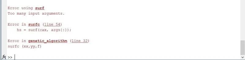
This error was occers when I mistakely give name a of file
RESULTS / OUTPUTS :
Study 1 : -
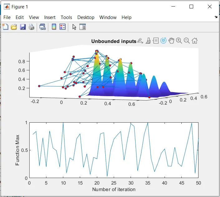
The results obtained for the unbounded inputs vary over a large sized interval. Thus , providing a varge idea of the global maxima . But it can be observes that the value of 'F MAXIMUM' lies between the interval [0,1] . Therefore, we can give more precise results .
Study 2 :-
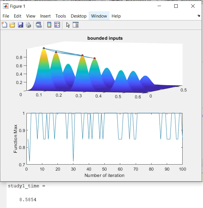
STUDY 3:-
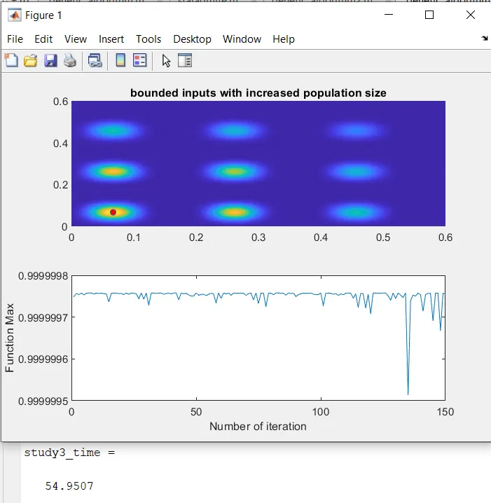
The use 'POPULATION METHOD ' with in boumded inputs increases the probability of determing the exact value of the Global Maxima . Assumed value of poplation size is 550.
CONCLUSION : The Global Maxima is calculated by Population Sizing and the plots provide a visual contest of the solution and verifies the authenticity of the obtained value .
REFERENCES :
1.https://www.sciencedirect.com/topics/engineering/genetic-algorithm
2.https://www.tutorialspoint.com/genetic_algorithms/genetic_algorithms_introduction.htm