Week 5 - Curve fitting

Aim: Writing Python code to fit a linear and cubic polynomial for the Cp data with explanation of results and explaining the parameters used to measure the fitness characteristics for both the curves.

Objective:

• Explaining the meaning of ‘popt’ and ‘pcov’.
• Explaining about np. array(temperature)
• Explaining the meaning of the * in *popt.
• Writing the code to fit a linear and cubic polynomial for the Cp data. Explaining if your results are good or bad.
• Explaining needs to be done in order to make the curve fit perfect
• Showing how well the plotted curve has been fit empirically

Objective #1: Meaning of ‘popt’ and ‘pcov’.

'popt'- Generally refers to an array of optimal readings or values for the given declared parameters which helps to minimize the sum of the squares of the leftover values.

'pcov'- A two-dimensionally array that contains the estimated covariance of popt. The diagonals provide the variance of the parameter estimate.

Objective #2: Explaining about np. array(temperature)

‘np.array(temperature)’ - The function that stores the values of the temperature as an array and then passes it to the ‘numpy’ function.

Objective #3: Explaining the meaning of the * in *popt.

'popt' indicates and returns each coefficient (i.e.: a,b,c etc.) stored in ‘popt’ array.

Objective #4: Writing the code to fit a linear and cubic polynomial for the Cp data. Explaining if your results are good or bad.

Python Code:

'''

Challenge-5 - Curve Fitting

'''

import math

import numpy as np

import matplotlib.pyplot as plt

from scipy.optimize import curve_fit

# Curve fit function - Linear Polynomial

def func1(t, a, b):

return a*t + b # Linear Polynomial equation

# Curve fit function - Cubic Polynomial

def func2(t, a, b, c, d):

return a*pow(t,3)+b*pow(t,2) + c*t + d # Cubic Polynomial equation

# Reading thermodynamic data file

def read_file():

temperature = [] # Empty array for temperature

cp =[] # Empty array for specific heat

for line in open('data', 'r'): # calling the file 'data' to read data

values = line.split(',') # split the each line by ','

# 1st value, index 0 and converting strigns into floats

# Store the values in exmpty array temperature = [] for each iteration

temperature.append(float(values[0]))

# 2nd value, index 1 and converting strigns into floats

# Store the values in exmpty array cp=[] for each iteration

cp.append(float(values[1]))

return [temperature, cp] # retuen the values to the fucntion

# Linear Curve Fitting

# Main program

temperature, cp = read_file()

# popt - coeffciets a,b,c

popt1, pcov1 = curve_fit(func1, temperature, cp)

# calculating fit cp values using the coefficients with temperature values

fit_cp_lin = func1(np.array(temperature), *popt1)

# Cubic Curve Fitting

# Main program

# temperature, cp = read_file()

# popt - coeffciets a,b,c

popt2, pcov2 = curve_fit(func2, temperature, cp)

# calculating fit cp values using the coefficients with temperature values

fit_cp_cubic = func2(np.array(temperature), *popt2)

# plotting

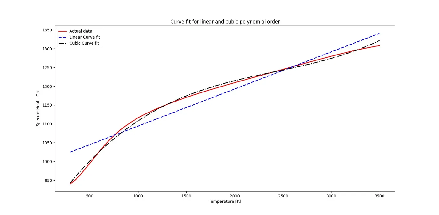
plt.plot(temperature, cp,'r', linewidth=2)

plt.plot(temperature, fit_cp_lin,'b--', Linewidth=2) # plotting linear curve fit

plt.plot(temperature, fit_cp_cubic,'k-.', Linewidth=2) # plotting cubic curve fit

plt.legend(['Actual data', 'Linear Curve fit','Cubic Curve fit'])

plt.title('Curve fit for linear and cubic polynomial order')

plt.xlabel('Temperature [K]')

plt.ylabel('Specific Heat - Cp')

plt.show()

# Calculation of Goodness of Fit.

# The sum of squares due to error(SSE)

a = np.size(cp)

for i in range(a):

sse_linear = pow((cp-fit_cp_lin),2)# Calculating SSE errors at every value for Linear Predicted Curve

sse_cubic = pow((cp-fit_cp_cubic),2)# Calculating SSE errors at every value for Cubic Predicted Curve

SSE_linear = np.sum(sse_linear)

SSE_cubic = np.sum(sse_cubic)

# 2.R-Square.

Mean = (np.sum(cp) / len(cp)) # Calculating mean value of cp data

print('Mean of Cp:',Mean) # printing the mean values of specific heat Cp

for i in range(a):

ssr_linear = pow((fit_cp_lin-Mean),2)# Calculating SSE errors at every value for Linear Predicted Curve

ssr_cubic = pow((fit_cp_cubic-Mean),2)# Calculating SSE errors at every value for Cubic Predicted Curve

SSR_linear = np.sum(ssr_linear) # Sum of SSR error of each value of Linear Predicted Curve

SST_linear = SSR_linear + SSE_linear # Calculating SST value for Linear Predicted Curve

Rsq_linear = SSR_linear / SST_linear # Calculating R-Square error value of Linear Predicted Curve

SSR_cubic = np.sum(ssr_cubic) # Sum of SSR error of each value of Cubic Predicted Curve

SST_cubic = SSR_cubic + SSE_cubic # Calculating SST value for Cubic Predicted Curve

Rsq_cubic = SSR_cubic / SST_cubic # Calculating R-Square errors at every value for Cubic Predicted Curve

# 3.Root mean square error(RMSE).

RMSE_linear = math.sqrt(SSE_linear / len(cp)); # Calculating RMSE error value of Linear Predicted Curve.

RMSE_cubic = math.sqrt(SSE_cubic / len(cp)); # Calculating RMSE error value of Cubic Predicted Curve.

# 4.Adjusted R-Square

K_linear = len(popt1)-1 # Calculating No of independent variables in Linear Predicted Curve

X = pow(Rsq_linear,2)

Rsq_adj_linear = (1-[(1-X)*(len(cp)-1)/(len(cp)-K_linear-1)]) # Calculating Adjusted_R-Square value of Linear Predicted Curve

K_cubic = len(popt2)-1 # Calculating No of independent variables in Cubic Predicted Curve

Y = pow(Rsq_cubic,2)

Rsq_adj_cubic = (1-[(1-Y)*(len(cp)-1)/(len(cp)-K_cubic-1)]) # Calculating Adjusted_R-Square value of Cubic Predicted Curve

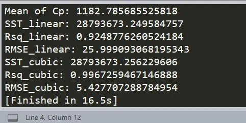
print('SST_linear:',SST_linear)

print('Rsq_linear:',Rsq_linear)

print('RMSE_linear:',RMSE_linear)

print('SST_cubic:',SST_cubic)

print('Rsq_cubic:',Rsq_cubic)

print('RMSE_cubic:',RMSE_cubic)

Snaps of the python code:

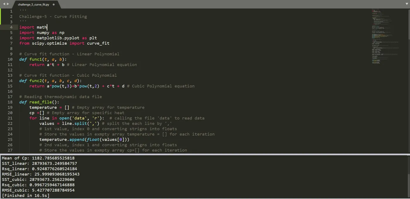
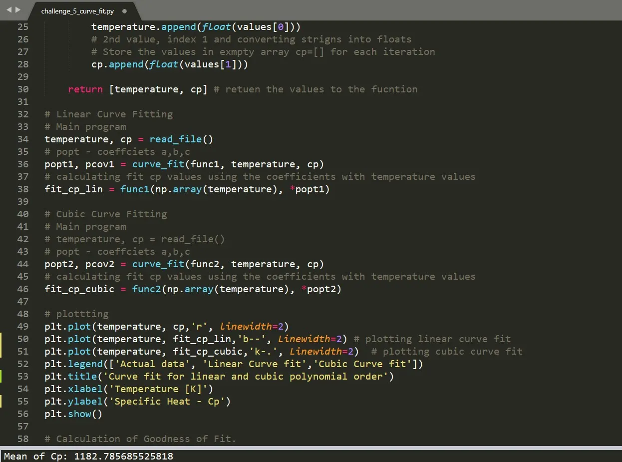
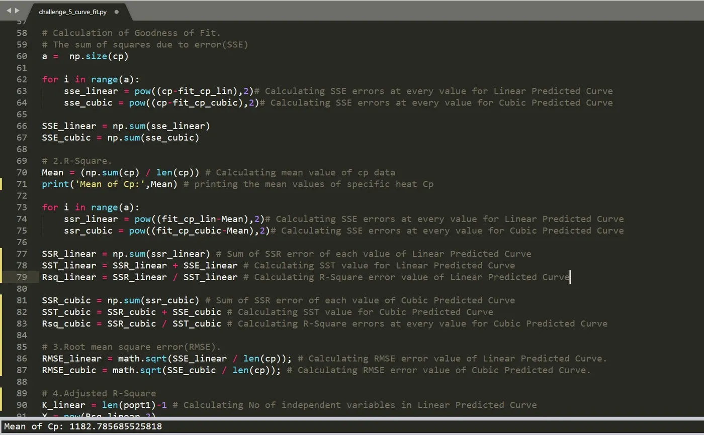
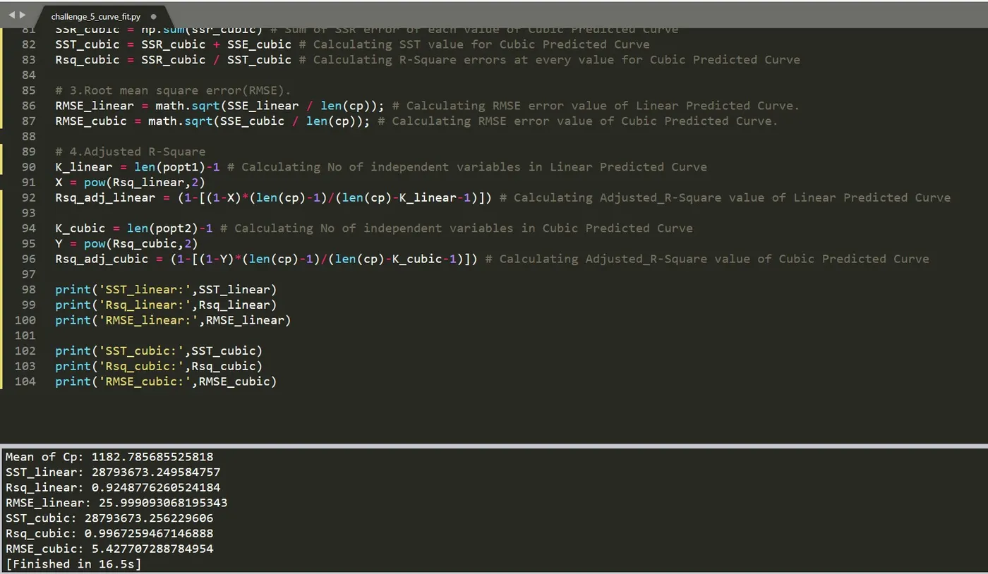
Code Explanation:

• Initially, necessary modules such as 'math', 'matplotlib', 'Numpy', 'scipy' are imported to perform their respective functions.
• Two functions are defined which return linear and cubic equations.
• The following data is loaded into Python by placing it in the right directory and a function read_file is created. For loop is used to run each line by using 'open' command with 'r' to read it.
• From the data obtained, two individual column matrices of temperature and specific heat are derived.
• For curve fitting, 'popt' and 'pcov' are used as output fostoring parameters obtained by 'curve_fit' command which takes input as the required
• unction(linear or cubic) , temperature, and Cp. Now, another variable named 'fit_cp' stores the new values of Cp calculated by using temperature array.
• Plots of both raw dataset and predicted dataset are made and compared to find fitness characteristics for both the curves for both linear and cubic polynomial.
• Fitness characteristics are calculated to show the results good or bad

Output:

#1 Curve fit Plot

Inference:

It is observed that the increase in degree of polynomial gives us the prefect curve fit. Thus, in the given problem cubic curves can be made as best fits.

#2 Error Values:

Inference:

The adjusted R-square statistic can take on any value less than or equal to 1, with a value closer to 1 indicating a better fit.

Objective #5: Explaining needs to be done in order to make the curve fit perfect

• By increasing the order of the polynomial (Cubic Polynomial -3^rd order), the curve fits perfectly to the original data.
• If Curve fit perfectly to the set to the original data without any errors we can consider as perfectly fitted curves.

Objective #6: Showing how well the plotted curve has been fit empirically

Goodness of Fit -

Parameters that used to measure the fitness characterizes of both the actual and curve fitted curves

• The sum of squares due to error (SSE)
• R-square
• Degrees of freedom for error (DFE)
• Adjusted R-square
• Root mean squared error (RMSE)

Sum of Squares Due to Error

This statistic measures the total deviation of the response values from the fit to the response values. It is also called the summed square of residuals and is usually labelled as SSE.

SSE=n∑i=1wi(yi−ˆyi)2

A value closer to 0 indicates that the model has a smaller random error component, and that the fit will be more useful for prediction.

R-Square

This statistic measures how successful the fit is in explaining the variation of the data. Put another way, R-square is the square of the correlation between the response values and the predicted response values. It is also called the square of the multiple correlation coefficient and the coefficient of multiple determination.

R-square is defined as the ratio of the sum of squares of the regression (SSR) and the total sum of squares (SST). SSR is defined as

SSR=n∑i=1wi(ˆyi−‾y)2

SST is also called the sum of squares about the mean, and is defined as

SST=n∑i=1wi(yi−‾y)2

where SST = SSR + SSE. Given these definitions, R-square is expressed as

R-square=SSRSST=1−SSESST

R-square can take on any value between 0 and 1, with a value closer to 1 indicating that a greater proportion of variance is accounted for by the model. For example, an R-square value of 0.8234 means that the fit explains 82.34% of the total variation in the data about the average.

If you increase the number of fitted coefficients in your model, R-square will increase although the fit may not improve in a practical sense. To avoid this situation, you should use the degrees of freedom adjusted R-square statistic described below.

Degrees of Freedom Adjusted R-Square

This statistic uses the R-square statistic defined above, and adjusts it based on the residual degrees of freedom. The residual degrees of freedom is defined as the number of response values n minus the number of fitted coefficients m estimated from the response values.

v = n – m

v indicates the number of independent pieces of information involving the n data points that are required to calculate the sum of squares. Note that if parameters are bounded and one or more of the estimates are at their bounds, then those estimates are regarded as fixed. The degrees of freedom is increased by the number of such parameters.

The adjusted R-square statistic is generally the best indicator of the fit quality when you compare two models that are nested — that is, a series of models each of which adds additional coefficients to the previous model.

adjusted R-square=1−SSE(n−1)SST(v)

The adjusted R-square statistic can take on any value less than or equal to 1, with a value closer to 1 indicating a better fit. Negative values can occur when the model contains terms that do not help to predict the response.

Root Mean Squared Error(RMSE)

This statistic is also known as the fit standard error and the standard error of the regression. It is an estimate of the standard deviation of the random component in the data, and is defined as

RMSE=s=√MSE

where MSE is the mean square error or the residual mean square

MSE=SSEv

Just as with SSE, an MSE value closer to 0 indicates a fit that is more useful for prediction.

Results:

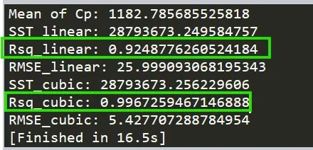
From above goodness of fit error calculation, we see the value of R - Square for linear curve fit is 0.924 and R - Square for cubic curve fit is 0.996.

So, R-square statistic can take on any value less than or equal to 1, with a value closer to 1 indicating a better fit.