Week 5 - Curve fitting

1. What do popt and pcov mean?

In the context of curve_fit(func, temperature, cp) (from the scipy.optimize library in Python), popt and pcov are:

• popt: Optimal values of the parameters that minimize the difference between the curve defined by func and the cp data. These are the best-fit parameters for the function func that you are trying to fit to the temperature and Cp data.

• pcov: The covariance of popt, which gives an estimate of the uncertainty of the parameter estimates in popt. The diagonal elements of pcov are the variances of the fitted parameters, and the off-diagonal elements provide the covariance between pairs of parameters.

2. What does np.array(temperature) do?

np.array(temperature) converts the list or iterable temperature into a NumPy array. NumPy arrays are more efficient for numerical operations and enable vectorized operations, which is why they are commonly used in scientific computing.

For example, if temperature is a list of temperature values, calling np.array(temperature) will transform it into an array that supports mathematical operations and matrix manipulations.

3. What does the * in *popt mean?

The * operator in *popt is used to unpack the values in the popt array. When popt contains multiple values (such as coefficients for a curve fit), using *popt will pass each value as an individual argument to a function.

For example, if popt contains three values [a, b, c] for fitting a cubic polynomial, then *popt will unpack these values as func(x, a, b, c).

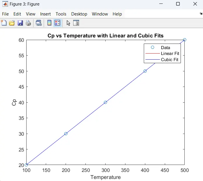
4. MATLAB code to fit a linear and cubic polynomial for Cp data

Here's an example of how you can fit a linear and cubic polynomial to Cp data in MATLAB:

MATLAB Code:

% Assuming you have your temperature (x) and Cp (y) data

% Linear fit (degree 1)

p1 = polyfit(temperature, cp, 1); % Linear fit

cp_linear = polyval(p1, temperature); % Evaluate the fit

% Cubic fit (degree 3)

p3 = polyfit(temperature, cp, 3); % Cubic fit

cp_cubic = polyval(p3, temperature); % Evaluate the fit

% Plot the data and fits

figure;

plot(temperature, cp, 'o', 'DisplayName', 'Data'); % Original data

hold on;

plot(temperature, cp_linear, '-r', 'DisplayName', 'Linear Fit');

plot(temperature, cp_cubic, '-b', 'DisplayName', 'Cubic Fit');

legend;

xlabel('Temperature');

ylabel('Cp');

title('Cp vs Temperature with Linear and Cubic Fits');

hold off;

Explanation of Results:

• Linear Fit: This is a straight-line approximation (degree 1). If the data has a clear linear trend, this should fit well, but if there is curvature in the data, the linear fit will not be accurate.

• Cubic Fit: This is a higher-order polynomial (degree 3), which can capture more complex behaviors in the data. It may provide a better fit if the Cp data shows non-linear trends.

To assess the goodness of fit, you would calculate metrics like R², residuals, or visually inspect the curve and how well it follows the data points.

5. What needs to be done to make the curve fit perfect?

To make the curve fit "perfect," here are a few considerations:

• Use a Higher-Order Polynomial: If your data is highly non-linear, increasing the degree of the polynomial can lead to a better fit. However, this risks overfitting, where the curve fits the noise in the data rather than the true underlying trend.

• Use a More Appropriate Model: Instead of forcing a polynomial, consider using a model that better captures the physical behavior of Cp with temperature. For example, empirical or thermodynamic models might provide a better fit than simple polynomials.

• Collect More Data: Having more data points across the temperature range can reduce the variability in the curve fit.

6. How to empirically show how well your curve has been fit?

Empirically, you can evaluate how well the curve fits using:

• Residual Plot: Plot the residuals (the difference between the observed Cp values and the predicted Cp values from the fit). If the residuals show no pattern (i.e., they are randomly scattered around zero), this indicates a good fit.

• Goodness-of-Fit Metrics: Calculate metrics such as:

  • R² (coefficient of determination): Measures how well the data fits the model. R² values close to 1 indicate a good fit.
  • RMSE (Root Mean Squared Error): Measures the average magnitude of the error between the data points and the fitted model.

In MATLAB, you can calculate these metrics like this:

MATLAB Code for R² and RMSE:

% Compute residuals for linear and cubic fits

residuals_linear = cp - cp_linear;

residuals_cubic = cp - cp_cubic;

% Total sum of squares

ss_total = sum((cp - mean(cp)).^2);

% Sum of squares of residuals (for each fit)

ss_res_linear = sum(residuals_linear.^2);

ss_res_cubic = sum(residuals_cubic.^2);

% R-squared values

r_squared_linear = 1 - (ss_res_linear / ss_total);

r_squared_cubic = 1 - (ss_res_cubic / ss_total);

% Display R-squared values

fprintf('R-squared (Linear Fit): %.4f\n', r_squared_linear);

fprintf('R-squared (Cubic Fit): %.4f\n', r_squared_cubic);

R-squared (Linear Fit): 1.0000

R-squared (Cubic Fit): 1.0000