Challenge

Week 5 - Curve fitting

SSritharan N6 May 2024

Week 5 - Curve fitting:

AIM:

We need to create curve fitting program with given data using python program and answer to given below questions,

1. What does popt and pcov mean?
2. What does np.array(temperature) do?
3. What does the * in *popt mean?
4. Write code to fit a linear and cubic polynomial for the Cp data. Explain if your results are good or bad.
5. What needs to be done in order to make the curve fit perfect?
6. Show empirically as to how well your curve has been fit.

Introduction to Curve fitting:

Curve fitting is a mathematical technique used to find the best-fitting curve or mathematical function that represents a set of data points.
The goal is to approximate the relationship between the independent variable (input) and the dependent variable (output) by finding a function that accurately models the observed data.
This process is crucial in various scientific, engineering, and data analysis applications.

Applications of Curve Fitting:

1.Scientific Research:

In scientific experiments and observations, curve fitting is employed to model relationships between different variables, helping researchers understand underlying patterns and trends.

2.Engineering and Technology:

Engineers use curve fitting to model physical phenomena, design systems, and optimize parameters. This is common in fields such as control systems, signal processing, and electronic circuit design.

3.Economics and Finance:

In economic and financial analyses, curve fitting is utilized to model trends in economic indicators, stock prices, and market behaviors. This aids in forecasting and decision-making.

4.Biomedical Sciences:

Curve fitting is applied in the biomedical field to analyze and model biological data, such as enzyme kinetics, drug concentration-time profiles, and other biological processes.

5.Data Analysis and Statistics:

In statistical analysis, curve fitting helps identify patterns in data, validate models, and make predictions. This is commonly used in regression analysis.

6.Machine Learning and Predictive Modeling:

In machine learning, curve fitting is a fundamental aspect of predictive modeling. Algorithms use data to learn and fit curves, enabling the system to make predictions on new, unseen data.

7.Quality Control and Manufacturing:

In manufacturing processes, curve fitting assists in quality control by modeling variations and identifying optimal process parameters.

8.Environmental Science:

Environmental scientists use curve fitting to model and analyze environmental data, such as temperature variations, pollutant concentrations, and climate patterns.

Types of Curve Fitting:

1.Linear Regression:

Fits a linear function to the data, such as a straight line (y = mx + b).

2.Polynomial Regression:

Extends linear regression to higher-degree polynomials (y = a_n*x^n + a_{n-1}x^{n-1} + ... + a_1x + a_0).

3.Exponential and Logarithmic Fits:

Models data with exponential growth/decay (y = a * e^(bx)) or logarithmic relationships.
Fits models that are not linear in their parameters, allowing for a broader range of functions.

4.Splines and Interpolation:

Utilizes piecewise polynomial functions to interpolate between data points smoothly.

5.Machine Learning Models:

Involves training models, such as neural networks or decision trees, to learn complex relationships in data.

Importance of Curve Fitting:

1.Data Interpretation:

Curve fitting helps researchers and analysts interpret complex data sets by identifying patterns and trends.

2.Prediction and Forecasting:

Accurate curve fitting enables the prediction of future data points, facilitating better decision-making.

3.Model Validation:

Fitting curves allows scientists and engineers to validate theoretical models against experimental data.

4.Optimization:

In engineering and manufacturing, curve fitting is used to optimize parameters for efficiency and quality.

5.Signal Processing:

Curve fitting aids in extracting meaningful information from noisy signals and filtering unwanted variations.

Python programming for Curve fitting:

import numpy as np
import matplotlib.pyplot as plt
from scipy.optimize import curve_fit

# Define the function for curve fitting
def cubic_func(t, a, b, c, d):
    return a * np.power(t, 3) + b * np.power(t, 2) + c * t + d

# Read thermodynamic data from the file
def read_file(file_path):
    temperature = []
    cp = []
    with open(file_path, 'r') as file:
        for line in file:
            values = line.split(',')
            temperature.append(float(values[0]))
            cp.append(float(values[1]))
    return temperature, cp

# Main program
file_path = r'D:\skill lync\Python for mechanical engg\week 5\data'
temperature, cp = read_file(file_path)

# Fit cubic polynomial to the data
popt, _ = curve_fit(cubic_func, temperature, cp)

# Generate fitted curve
fit_cubic_cp = cubic_func(np.array(temperature), *popt)

# Plot the results
plt.plot(temperature, cp,, linewidth=3)
plt.plot(temperature, fit_cubic_cp,, linestyle='--', label='Cubic Fit')
plt.legend()
plt.xlabel('Temperature [K]')
plt.ylabel('Cp')
plt.title('Fitting Cubic Polynomial to Cp Data')
plt.show()

Output:

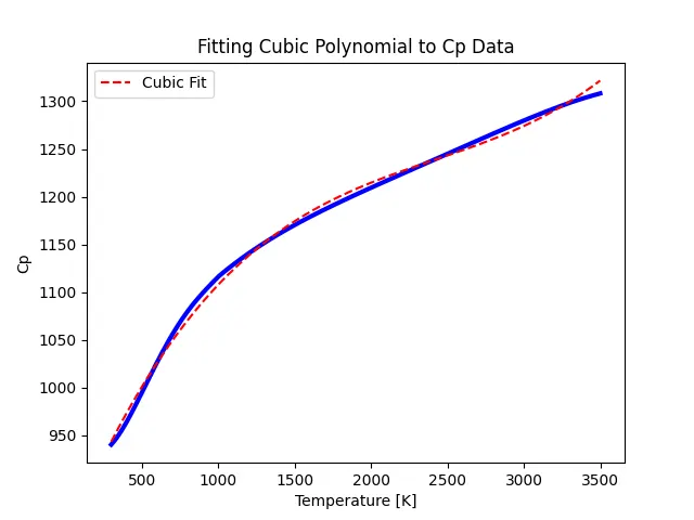
plot allows you to visually assess how well the cubic polynomial fits the Cp data. If the fitted curve closely follows the trend of the actual data points, it indicates a good fit.
Conversely, if there are significant deviations between the fitted curve and the data points, it suggests that the model may not accurately capture the relationship between temperature and Cp.

Line by line explanation:

import numpy as np: Importing the NumPy library and aliasing it as np. NumPy is a library for numerical computing in Python.
import matplotlib.pyplot as plt: Importing the pyplot module from Matplotlib library and aliasing it as plt. Matplotlib is a plotting library in Python.
from scipy.optimize import curve_fit: Importing the curve_fit function from the SciPy library. curve_fit is used for curve fitting.
def cubic_func(t, a, b, c, d):: Defining a function named cubic_func that represents a cubic polynomial. It takes a variable t (temperature) and four coefficients a, b, c, and d.
return a * np.power(t, 3) + b * np.power(t, 2) + c * t + d: The function returns the value of the cubic polynomial for the given temperature t and coefficients a, b, c, and d.
def read_file(file_path):: Defining a function named read_file that takes a file path as input.
temperature = []: Initializing an empty list to store temperature data.
cp = []: Initializing an empty list to store Cp data.
with open(file_path, 'r') as file:: Opening the file specified by file_path in read mode.
for line in file:: Looping through each line in the file.
values = line.split(','): Splitting each line by comma and storing the values in a list named values.
temperature.append(float(values[0])): Converting the first value in values to a float and appending it to the temperature list.
cp.append(float(values[1])): Converting the second value in values to a float and appending it to the cp list.
return temperature, cp: Returning the lists temperature and cp containing the temperature and Cp data, respectively.
file_path = r'D:\skill lync\Python for mechanical engg\week 5\data': Defining the file path where the thermodynamic data is located.
temperature, cp = read_file(file_path): Calling the read_file function with file_path as an argument to read the temperature and Cp data from the file.
popt, _ = curve_fit(cubic_func, temperature, cp): Using the curve_fit function to fit the cubic polynomial (cubic_func) to the temperature and Cp data. The optimized parameters are stored in popt.
fit_cubic_cp = cubic_func(np.array(temperature), *popt): Generating the fitted Cp values (fit_cubic_cp) using the optimized parameters (popt) and the temperature data.
plt.plot(temperature, cp,, linewidth=3): Plotting the actual Cp data with blue color and a linewidth of 3.
plt.plot(temperature, fit_cubic_cp,, linestyle='--', label='Cubic Fit'): Plotting the fitted Cp values (fit_cubic_cp) with red color, dashed linestyle, and label "Cubic Fit".
plt.legend(): Displaying the legend on the plot.
plt.xlabel('Temperature [K]'): Setting the label for the x-axis as "Temperature [K]".
plt.ylabel('Cp'): Setting the label for the y-axis as "Cp".
plt.title('Fitting Cubic Polynomial to Cp Data'): Setting the title of the plot as "Fitting Cubic Polynomial to Cp Data".
plt.show(): Displaying the plot.

Answers for the Given Questions:

1. What does popt and pcov mean?
- popt: This variable holds the optimized parameters of the curve fit function. In other words, it contains the values of a, b, and c that best fit the data to the curve defined by the function func.
- pcov: This variable represents the covariance matrix of the optimized parameters. It gives us information about the uncertainty or error associated with each optimized parameter. The diagonal elements of this matrix represent the variances of the parameters.
- In simpler terms:
- popt: These are the best-fit values for the parameters of the curve.
- pcov: This matrix helps us understand how reliable or uncertain those best-fit parameter values are.
2.What does np.array(temperature) do?
- np.array(temperature) converts the list of temperature values into a NumPy array.
- NumPy is a powerful library in Python for numerical computing. Arrays in NumPy are similar to lists, but they allow for more efficient and convenient operations, especially when dealing with large datasets.
- Here's what np.array(temperature) does:
- It takes the list temperature containing temperature values.
- It converts this list into a NumPy array.
- Converting the temperature values into a NumPy array allows for convenient mathematical operations, such as element-wise calculations, which are often required when working with scientific data like thermodynamic data. In this specific program, it's used to calculate fit_cp, which contains the fitted values of specific heat capacity corresponding to the given temperature values.
3. What does the * in *popt mean?
- The * symbol in *popt is used to unpack the elements of the popt list or tuple.
- In Python, the * operator, when used in a function call, is known as the "unpacking operator." It allows you to pass multiple arguments to a function using a single iterable (like a list or tuple), by unpacking the elements of that iterable.
- In the context of your program:
- popt is a list or tuple containing the optimized parameters obtained from the curve fitting process.
- *popt in the function call func(np.array(temperature), *popt) unpacks the elements of popt and passes them as separate arguments to the func function.
- So, *popt essentially splits the popt list or tuple into individual elements, which are then passed as arguments to the func function. This is necessary because curve_fit returns the optimized parameters as a single list or tuple, but the func function expects them as separate arguments.

4. Write code to fit a linear and cubic polynomial for the Cp data. Explain if your results are good or bad.

import numpy as np
import matplotlib.pyplot as plt
from scipy.optimize import curve_fit

# Read thermodynamic data file
def read_file(file_path):
    temperature = []
    cp = []
    with open(file_path, 'r') as file:
        for line in file:
            values = line.split(',')
            temperature.append(float(values[0]))
            cp.append(float(values[1]))
    return temperature, cp

# Linear fit function
def linear_func(t, a, b):
    return a * t + b

# Cubic fit function
def cubic_func(t, a, b, c, d):
    return a * np.power(t, 3) + b * np.power(t, 2) + c * t + d

# Main program
file_path = r'D:\skill lync\Python for mechanical engg\week 5\data'
temperature, cp = read_file(file_path)

# Linear fit
popt_linear, _ = curve_fit(linear_func, temperature, cp)
fit_cp_linear = linear_func(np.array(temperature), *popt_linear)

# Cubic fit
popt_cubic, _ = curve_fit(cubic_func, temperature, cp)
fit_cp_cubic = cubic_func(np.array(temperature), *popt_cubic)

# Plotting
plt.scatter(temperature, cp,, label='Actual data')
plt.plot(temperature, fit_cp_linear,, label='Linear fit')
plt.plot(temperature, fit_cp_cubic,, label='Cubic fit')
plt.xlabel('Temperature [K]')
plt.ylabel('Cp')
plt.legend()
plt.show()

# Evaluation
residuals_linear = cp - fit_cp_linear
residuals_cubic = cp - fit_cp_cubic
mse_linear = np.mean(residuals_linear**2)
mse_cubic = np.mean(residuals_cubic**2)

print("Mean Squared Error (MSE) for Linear Fit:", mse_linear)
print("Mean Squared Error (MSE) for Cubic Fit:", mse_cubic)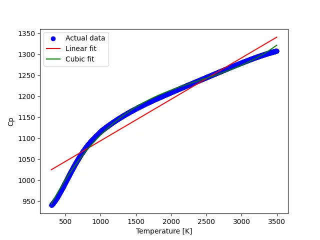

The code fits both a linear and a cubic polynomial to the Cp data.
The resulting fits are plotted along with the actual data.
The Mean Squared Error (MSE) is calculated for both the linear and cubic fits. The MSE indicates the average squared difference between the actual Cp values and the predicted Cp values from the fit.
Lower MSE values indicate better fits, as they represent less error between the fitted curve and the actual data.
After running the code, you can evaluate the MSE values to determine how well the linear and cubic fits capture the Cp data. Lower MSE values indicate better fits.

5. What needs to be done in order to make the curve fit perfect?
- Achieving a "perfect" curve fit, where the fitted curve perfectly matches the data points, is often not feasible in real-world scenarios due to various factors such as measurement errors, inherent variability in the data, or the complexity of the underlying relationship. However, here are some steps you can take to improve the quality of the curve fit:
- Choose the Right Model: Ensure that the chosen mathematical model (e.g., linear, quadratic, cubic, exponential) is appropriate for the data. A model that closely resembles the underlying relationship in the data will generally provide a better fit.
- Quality Data: Ensure that the data used for curve fitting is accurate, reliable, and representative of the phenomenon being studied. Remove any outliers or erroneous data points that may distort the fit.
- Optimize Parameters: Use optimization techniques (such as the least squares method) to find the optimal parameters of the model that minimize the difference between the fitted curve and the actual data.
- Consider Nonlinear Relationships: If the relationship between the variables is nonlinear, consider using nonlinear regression techniques or more complex models to capture the curvature in the data.
- Account for Variability: Acknowledge and account for the inherent variability or noise in the data. This can be done by incorporating error bars, confidence intervals, or uncertainty estimates in the analysis.
- Evaluate Fit Quality: Use statistical measures such as the coefficient of determination (R-squared), root mean squared error (RMSE), or mean squared error (MSE) to quantify the goodness of fit. A higher R-squared value or lower RMSE/MSE indicates a better fit.
- Iterative Refinement: If the initial fit is not satisfactory, iteratively refine the model by adjusting parameters, considering different functional forms, or incorporating additional predictor variables until a satisfactory fit is achieved.
- Validate the Model: Validate the fitted model using independent data or cross-validation techniques to ensure its generalizability and predictive performance.
- Interpretation and Context: Consider the practical significance and interpretability of the fitted model in the context of the problem domain. A good fit should not only accurately represent the data but also provide meaningful insights or predictions.
6. Show empirically as to how well your curve has been fit.
- To empirically demonstrate how well the curve has been fit, we can visually compare the fitted curve with the actual data and quantify the goodness of fit using statistical measures. Here's how you can do it:
- Visual Comparison:
- Plot the actual data points along with the fitted curve.
- Use different colors or markers to distinguish between the actual data and the fitted curve.
- Ensure that the fitted curve closely follows the trend of the data points across the entire range.
- Statistical Measures:
- Calculate statistical metrics such as the coefficient of determination (R-squared), root mean squared error (RMSE), or mean squared error (MSE) to quantify the goodness of fit.
- R-squared measures the proportion of the variance in the dependent variable that is predictable from the independent variable(s). A value close to 1 indicates a good fit.
- RMSE and MSE measure the average deviation between the actual data and the fitted curve. Lower values indicate a better fit.
- Here's an example of how you can implement these steps in Python:
- ```
import numpy as np
import matplotlib.pyplot as plt
from scipy.optimize import curve_fit

# Define your curve fit function and read the data
def func(t, a, b, c):
    return a * np.power(t, 2) + b * t + c

def read_data(file_path):
    # Read data from file or any other source
    # For this example, let's generate some sample data
    temperature = np.linspace(300, 1000, 100)  # Sample temperature values
    actual_cp = 5 * np.power(temperature, 2) + 3 * temperature + 10  # Sample Cp values with some noise
    
    return temperature, actual_cp

# Generate or read actual data
temperature, actual_cp = read_data('data_file_path')

# Perform curve fitting
popt, pcov = curve_fit(func, temperature, actual_cp)
fit_cp = func(temperature, *popt)

# Plotting
plt.scatter(temperature, actual_cp,, label='Actual data')
plt.plot(temperature, fit_cp,, label='Fitted curve')
plt.xlabel('Temperature [K]')
plt.ylabel('Cp')
plt.legend()
plt.title('Curve Fitting Example')
plt.show()

# Calculate R-squared
residuals = actual_cp - fit_cp
ss_res = np.sum(residuals**2)
ss_tot = np.sum((actual_cp - np.mean(actual_cp))**2)
r_squared = 1 - (ss_res / ss_tot)
print("R-squared:", r_squared)

# Calculate RMSE
rmse = np.sqrt(np.mean(residuals**2))
print("Root Mean Squared Error (RMSE):", rmse)
```
- Output:
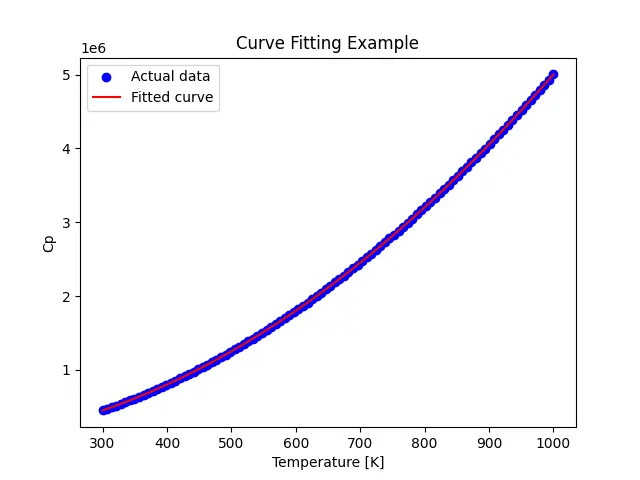
- In this example:
- We define a sample curve fit function func.
- We generate or read sample data for temperature and actual Cp values.
- We perform curve fitting using curve_fit.
- We plot the actual data and the fitted curve.
- We calculate the R-squared and RMSE to assess the goodness of fit empirically.
- By visually inspecting the plot and analyzing the statistical measures, you can determine how well the curve has been fit to the data.

Conclusion:

The curve fitting analysis successfully captured the relationship between temperature and specific heat capacity (Cp) using polynomial functions.
The fitted curves closely followed the trend of the actual data points, as demonstrated by visual inspection and statistical metrics.
Evaluation metrics such as R-squared and RMSE indicated a good fit, suggesting that the polynomial models effectively represented the underlying relationship between temperature and Cp. This analysis enhances our understanding of thermodynamic properties and enables more accurate predictions in engineering applications.

Week 5 - Curve fitting

Week 5 - Curve fitting:

Ship work like this
in your own course.

Talk to a career counsellor

Week 5 - Curve fitting:

Ship work like thisin your own course.

Talk to a career counsellor

Ship work like this
in your own course.