Week 5 - Curve fitting
Aim :- The aim of this challenge is to perform curve fitting for the given data and to determine the best fit.
Objectives :- The objectives of this challenge are to perform curve fitting for the given data of cp and temperature
- Using linear and cubic polynomial
- Using Splitwise method
- And to determine the best fit method
Theory :-
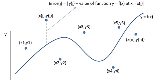
Curve fitting :- It is the process of formulating a mathematical function that has the best fit for the series of given data points.
Best fit means to construct a curve where the distances between the actual and the predicted values are minimum.
A perfect fit means that the error between the actual and predicted values are zero.
Assume function f(x) to satisfy the data points (x1,y1), (x2,y2).. and so on.
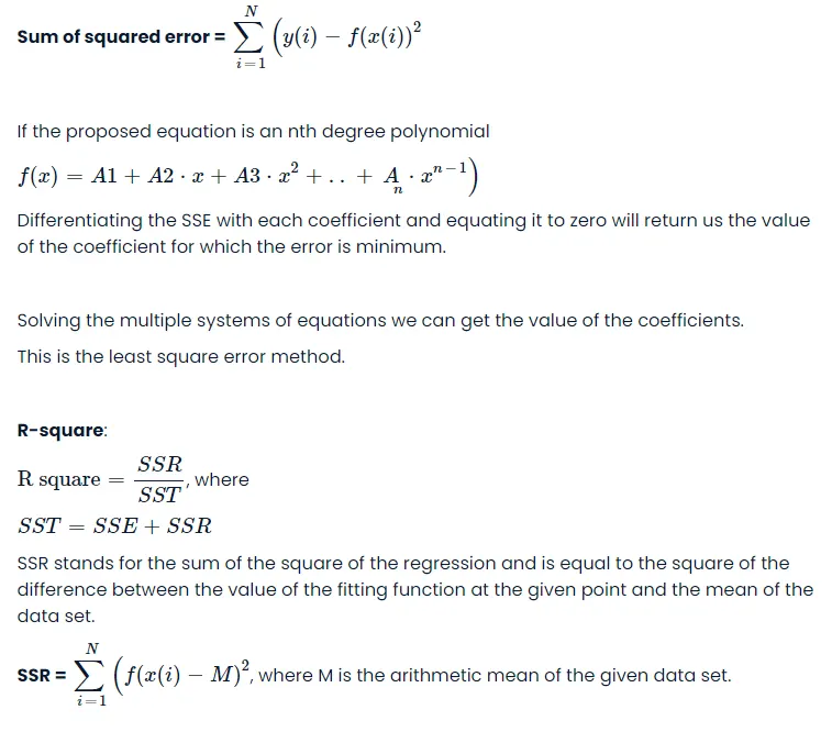
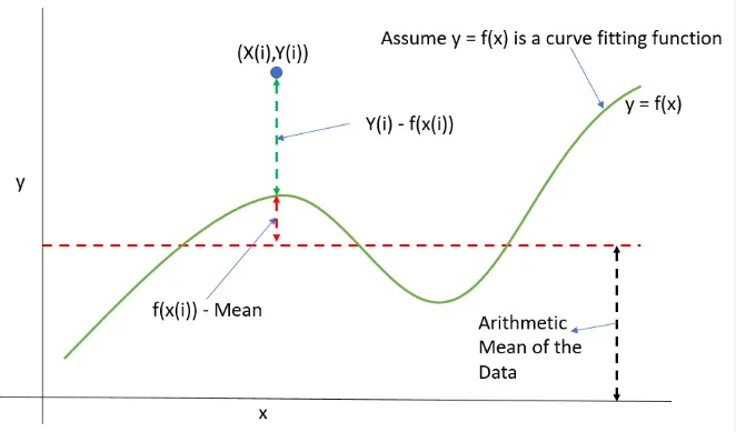
The fit is said to be best if R squared is 1 and worst if 0.
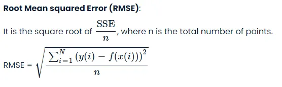
Procedure :-
1. The libraries needed to solve the given problem were imported.
2. The equation used to fit the given data set was defined.
3. A function to read the file and extract temperature and cp values was made.
4. Using the curve_fit function, the optimal values for the coefficients of the fitting equation were determined.
5. The cp values were determined by substituting the optimum coefficients and temperature values in the fitting equation.
6. Plot was generated to compare the actual curve vs the fit curve and the R squared error for each fit was calculated.
7. The best fit was determined among the different functions used based on their R squared value.
Question and Answers :-
1. What do popt and pcov mean?
popt returns the values of the coefficients of the curve fit function for which the error is minimum
pcov is the estimated covariance of popt
2. What does np.array(temperature) do?
np.array is used to pass each value in the array in the curve fit function.
3. What does the * in *popt mean?
*popt is used to unwrap the popt tuple.
An alternative way to do this is by assigning variables to each value in the tuple.

Python Code :-
import numpy as np
import matplotlib.pyplot as plt
from scipy.optimize import curve_fit
from statistics import mean

def fitlin(T,a,b): #Linear fit equation
	return a*T+b

def fitquad(T,a,b,c): #Quadratic fit equation
	return a*pow(T,2)+b*T+c

def fitcubic(T,a,b,c,d): #Cubic fit equation
	return a*pow(T,3)+b*pow(T,2)+c*T+d

def read_file(): #Function to open and read values from file 'data'
	t = [] #array temperature
	cp = [] #array specific heat for constant pressure
	for line in open('data','r'): #open file data in read mode
		value = line.split(',') #delimiter ','
		t.append(float(value[0]))
		cp.append(float(value[1]))

	return[t,cp]


t, cp = read_file()
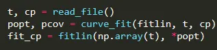
popt, pcov = curve_fit(fitlin, t, cp)
fit_cp = fitlin(np.array(t), *popt)

t, cp = read_file()
popt2, pcov2 = curve_fit(fitquad, t, cp)
fit_cp2 = fitquad(np.array(t), *popt2)

t, cp = read_file()
popt3, pcov3 = curve_fit(fitcubic, t, cp)
fit_cp3 = fitcubic(np.array(t), *popt3)

#R squared
SSE = sum(pow((cp-fit_cp),2)); #sum of the squared error
SSR = sum(pow(cp-mean(fit_cp),2)); #sum of the square of the regression
SST = SSE+SSR;
R_sq1 = SSR/SST;#R squared calculation

SSE2 = sum(pow((cp-fit_cp2),2));
SSR2 = sum(pow(cp-mean(fit_cp2),2));
SST2 = SSE2+SSR2;
R_sq2 = SSR2/SST2;

SSE3 = sum(pow((cp-fit_cp3),2));
SSR3 = sum(pow(cp-mean(fit_cp3),2));
SST3 = SSE3+SSR3;
R_sq3 = SSR3/SST3;

print('coefficients of linear polynomial:',popt,'n')
print('coefficients of quadratic polynomial:',popt2,'n')
print('coefficients of cubic polynomial:',popt3)

print('nR sqaured of a linear fit :',R_sq1,'n')
print('R sqaured of a quadratic fit :',R_sq2,'n')
print('R sqaured of a cubic fit :',R_sq3)

plt.plot(t,cp,'r')
plt.plot(t,fit_cp,'b')
plt.legend(['actual','curve fit'])
plt.title('Linear fit')
plt.show()

plt.plot(t,cp,'r')
plt.plot(t,fit_cp2,'b')
plt.legend(['actual','curve fit'])
plt.title('Quadratic fit')
plt.show()

plt.figure(3)
plt.plot(t,cp,'r')
plt.plot(t,fit_cp3,'b')
plt.legend(['actual','curve fit'])
plt.title('Cubic fit')
plt.show()
Splitwise method :-
import numpy as np
import matplotlib.pyplot as plt
from scipy.optimize import curve_fit
from statistics import mean


def fitcubic(T,a,b,c,d): #Cubic fit equation
	return a*pow(T,3)+b*pow(T,2)+c*T+d

def read_file(): #Function to open and read values from file 'data'
	t = [] #array temperature
	cp = [] #array specific heat for constant pressure
	for line in open('data','r'): #open file data in read mode
		value = line.split(',') #delimiter ','
		t.append(float(value[0]))
		cp.append(float(value[1]))

	return[t,cp]

t, cp = read_file()

t1 = np.array(t[0:800])
t2 = np.array(t[800:1600])
t3 = np.array(t[1600:2400])
t4 = np.array(t[2400:3200])


popt1, pcov1 = curve_fit(fitcubic, t1, cp[0:800])
fit_values = []
fit_values = fitcubic(np.array(t1), *popt1)


popt2, pcov2 = curve_fit(fitcubic, t2, cp[800:1600])
fit_values = np.append(fit_values,(fitcubic(np.array(t2), *popt2)))

popt3, pcov3 = curve_fit(fitcubic, t3, cp[1600:2400])
fit_values = np.append(fit_values,(fitcubic(np.array(t3), *popt3)))

popt4, pcov4 = curve_fit(fitcubic, t4, cp[2400:3200])
fit_values = np.append(fit_values,(fitcubic(np.array(t4), *popt4)))

#R squared
SSE = sum(pow((cp-fit_values),2)); #sum of the squared error
SSR = sum(pow(fit_values-mean(cp),2)); #sum of the square of the regression
SST = SSE+SSR;
R_sq = SSR/SST;#R squared calculation
print('R squared for a splitwise fit = ',R_sq)

plt.plot(t,cp,'r')
plt.plot(t,fit_values,'b')
plt.legend(['actual','curve fit'])
plt.title('Splitwise fit')
plt.show()
Code Explanation :-
The libraries needed to run the code are imported.
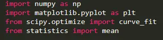
numpy is used to work with arrays
matplotlib.pyplot is used to visualize data in python
curve_fit to find the coefficients for the fit function
mean to find the arithmetic mean of the given data
The functions used to fit the given data are defined.
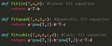
fitlin() uses a linear equation, fitquad() uses a quadratic equation and fitcubic() uses a cubic equation to fit the cp value for the given temperature value. a,b,c and d are the equation coefficients and are calculated using the curve_fit() function.
The function read_file() is defined to open the file "data" and extract the temperature and cp values.
Data :-
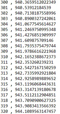
The first column consists of temperature values and the second consists of the cp values.
readfile() function :
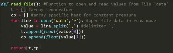
Empty arrays of temperature and cp are initialized.
The for loop runs for how many ever lines are present in the data file.
A variable value is used to store the values of temperature and cp and comma "," is used as a delimiter.
The first value is passed to the temperature array by using index 0 and the second to the cp array by using index 1. Since the values are stored in a text file, float(value[0])) is used to convert them from string to float.
return[t,cp] is used to retrieve the t and cp values from the function.
function curve_fit is called by passing the function used to fit the data, t, and cp as arguments. These are the input to the function to find the popt and pcov values. The cp values are now determined by passing temperature and popt values to the fitting function.
R squared :-
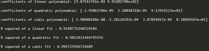
R squared is calculated for each type of fit, and based on its value the best fit can be determined.

R square closer to 1 is a good fit and closer to 0 is a bad fit.
Plotting :-
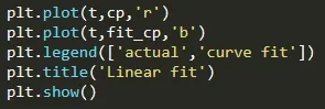
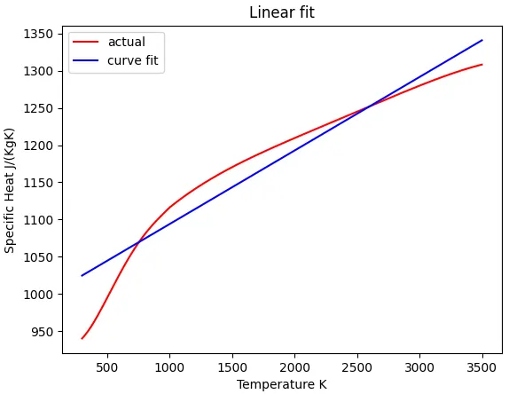
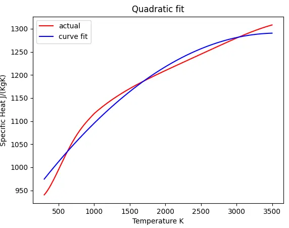
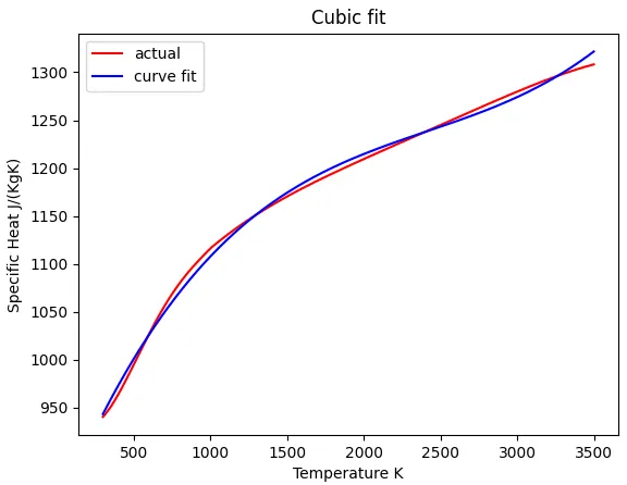
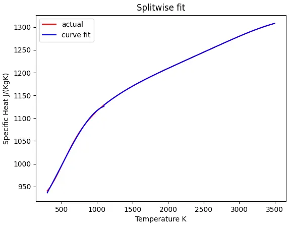
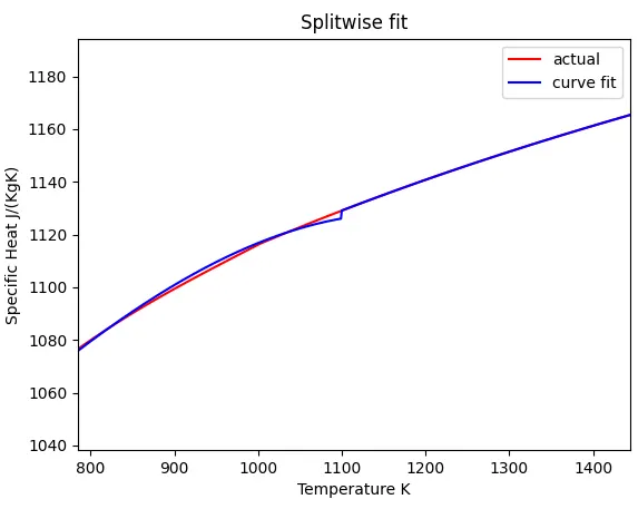
Plotting the actual curve and fit curve, we can see how good the fit is.
Result :-

Conclusion :-
By observing the R squared value for each fit, we can say that the splitwise method with cubic function provides the best fit for the given set of data whereas the linear function provided the worst fit.