Week 5 - Curve fitting

AIM: To write codes in Python to perform curve fitting.

OBJECTIVE :

1. To wite codes to fit a linear and cubic polynomial for the Cp data.
2. To plot the linear and cubic fit curves along with the raw data points.
3. To measure the fitness characteristics for both the curves.

THEORY: Curve fitting is the way we model or represent a data spread by assigning the best fit function (curve) along with the entire range. Ideally, it will capture the trend in the data and allow us to make predictions of how the data series will behave in the future.

Types of curve fitting include:

• Interpolation, where you discover a function that is an exact fit to the data points. Since this assumes no measurement error, it has limited applicability to real-life scenarios.
• Smoothing is when we find a function that is an approximate fit to the data points, but we give room for error and we allow our actual points to be near, but not necessarily on the line; given the error is minimized overall.

Linear and Polynomial Curve fitting :

(i) Linear curve fitting, or linear regression, is when the data is fit to a straight line. Although there might be some curve to your data, a straight line provides a reasonable enough fit to make predictions.

Since the equation of a generic straight line is always given by f(x)= a x + b, the question becomes: what a and b will give us the best fit line for our data?

Considering the vertical distance from each point to a prospective line as an error, and summing them up over our range, gives us a concrete number that expresses how far from ‘best’ the prospective line is.

A line that provides a minimum error can be considered the best straight line.

Since it’s the distance from our points to the line we’re interested in—whether it is positive or negative distance is not relevant—we square the distance in our error calculations. This also allows us to weight greater errors more heavily. So this method is called the least square approach.

(ii) Polynomial curve fitting is when we fit our data to the graph of a polynomial function. The same least-squares method can be used to find the polynomial, of a given degree, that has a minimum total error.

To choose the best fit for the curve the following four parameters help us to measure the goodness of fit criteria or how well the equations are representing the given datapoints:

1. The sum of squares due to error (SSESSE),
2. R-square (R2R2),
3. Adjusted R-squrae,
4. Root mean squared error (RMSERMSE)

GOVERNING EQUATIONS USED :

• Error = ∣y(i))−∣y(i))-value of f(x)f(x)at x(i)∣x(i)∣ = |y(i)−f(x(i))||y(i)-f(x(i))|,
• SSE (sum of squared error) = `S S E = ∑ n i = 1 [ Error ( i ) 2 ]`
• SSR (sum of square of regression) = n∑i=1(f(x(i))−Mean)2∑i=1n(f(x(i))-Mean)2,
• SST (sum of the squared total) = SSE+SSRSSE+SSR ,
• R2 ( R squared) = SSR/SST,
• RMSE (root mean squared error) = `R M S E = √ ( ∑ n i = 1 ( Y ( i ) − f ( x ( i ) ) ) 2 n = ) √ ( S S E n )`

where n is the total number of datapoints available.

Link of Data-https://drive.google.com/file/d/1vWi9Vj3AdQf0gqUK1u9jwS8zg92BHGR0/view?usp=sharing

code-

import math                                      #importing all the necessary libraries
import numpy as np
import matplotlib.pyplot as plt
from scipy.optimize import curve_fit


# Linear Curve fit function
def function_lcf(t, a, b):
    return a * t + b


# Cubic Curve fit function
def function_ccf(t, a, b, c, d):
    return a * pow(t, 3) + b * pow(t, 2) + c * t + d


# Reading thermodynamic data file
def read_file():                                  #creating a function for reading file
    temperature = []
    cp = []
    for line in open('data', 'r'):                #condition for getting all the data 
        values = line.split(',')
        temperature.append(float(values[0]))
        cp.append(float(values[1]))

    return [temperature, cp]


# Main Program 
#reading the file which is been accesed
temperature, cp = read_file()

popt, pcov = curve_fit(function_lcf, temperature, cp)
fit_cp_l = function_lcf(np.array(temperature), *popt) 
#plotting the graph of Temperature vs cp for linear curve fit
plt.figure(1)
plt.plot(temperature, cp, 'b--')
plt.plot(temperature, fit_cp_l, color='red')
plt.legend(['Actual data', 'Curve fit'])
plt.xlabel('Temperature (K)')
plt.ylabel('Cp')
plt.title('Linear Curve fitting')
plt.show()

popt, pcov = curve_fit(function_ccf, temperature, cp)
fit_cp_c = function_ccf(np.array(temperature), *popt)

#plotting the graph of temperature vs cp for cubic curve fit
plt.figure(2)
plt.plot(temperature, cp, 'b--')
plt.plot(temperature, fit_cp_c, color='red')
plt.legend(['Actual data', 'Curve fit'])
plt.xlabel('Temperature (K)')
plt.ylabel('Cp')
plt.title('Cubic Curve fitting')
plt.show()


#Measuring the fitness characetristics of the curves

s = np.sum(cp)
l = np.size(cp)
m = s / l # Finding mean of Cp data
print('Mean of all cp :', m)
print('') #This will print an empty line (use to give line break)

# For Linear curve fit
linear_sse = 0
linear_ssr = 0
for i in range(l):
    linear_error = abs((np.sum((cp[i] - fit_cp_l[i]))))
    linear_sse = linear_sse + pow(linear_error, 2)
    linear_ssr = linear_ssr + np.sum(pow((fit_cp_l[i] - m), 2))

print('For Linear Curve Fit')
linear_sst = linear_sse + linear_ssr
print('linear_sst :', linear_sst)
linear_R2 = linear_ssr / linear_sst
print('linear_R2 :', linear_R2)
linear_rmse = pow((linear_sse / l), 0.5)
print('linear_RMSE :', linear_rmse)
print('') #This will print an empty line (use to give line break)

# For Cubic curve fit
cubic_sse = 0
cubic_ssr = 0
for j in range(l):
    cubic_error = abs(np.sum((cp[i] - fit_cp_c[i])))
    cubic_sse = cubic_sse + (pow(cubic_error, 2))
    cubic_ssr = cubic_ssr + np.sum(pow((fit_cp_c[i] - m), 2))

print('For Cubic Curve Fit')
cubic_sst = cubic_sse + cubic_ssr
print('cubic_sst :', cubic_sst)
cubic_R2 = cubic_ssr / cubic_sst
print('cubic_R2 :', cubic_R2)
cubic_rmse = pow((cubic_sse / l), 0.5)
print('cubic_RMSE :', cubic_rmse)

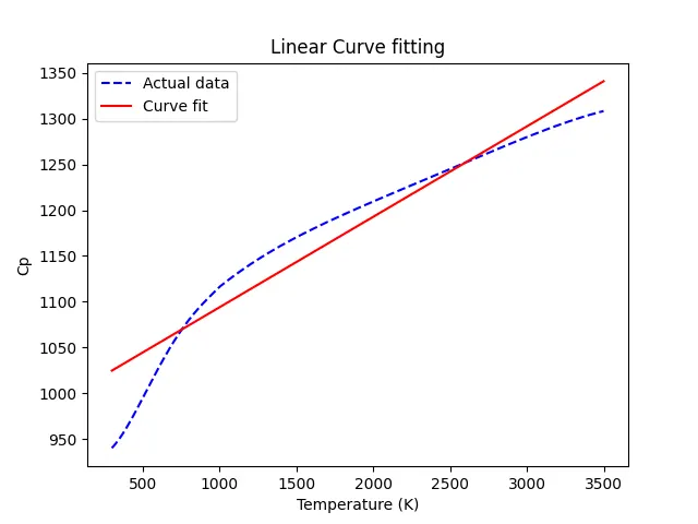
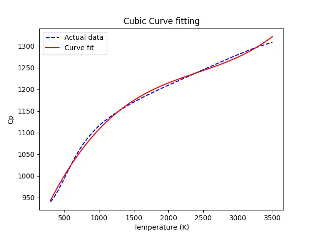
Graph-

Screenshot-

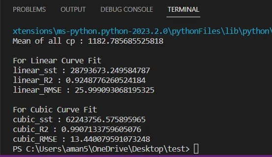
Result-

The values of R-Square (R2) is close to 1 for both linear and cubic curve which indicates the fit is a good fit.

Theory-

Q1. What does popt and pcov mean?

A1. ‘popt’ is an array that stores the values of the coefficients that are being passed in a given function.

‘pcov’ is a two-dimensional array that stores the values of the estimated covariance of ‘popt’ i.e the coefficients.

Q2. What does np.array(temperature) do?

A2. This command converts each value of temperature in the data file into an array using the NumPy module.

Q3. What does the * in *popt mean?

A3. '*' in ‘*popt' indicates and returns each coefficient stored in popt array.

Q4. What needs to be done in order to make the curve fit perfect?

A4. In order to make the curve fit perfect we can increase the order of the polynomial or break the data set into different groups of certain range or both.