Week 3 - Solving second order ODEs

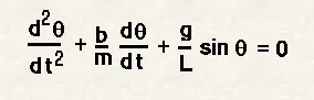
Aim: To write a program that solves the following ODE. This ODE represents the equation of motion of a simple pendulum with damping

Governing Equations:

In the above equation,

b is the damping coefficient. No units

m = mass of the ball in kg,

g is the gravitational acceleration. Units m/s^2

L is the pendulum’s length

Equation Description: The governing equations is an ordinary differential equation of a simple pendulum. Using this equation, we can find the oscillations of the pendulum and make an animation for it.

Physics behind the equation: Damping is a prominent phenomenon in everyday life. Examples of damping include Springs, wall clocks, etc. In a pendulum, the bob’s position with respect to time can be given by an ODE.

Objectives: The main objective of the project is to write a program to simulate a simple pendulum’s motion.

Firstly, we have to get all the values required like the lengths, angle, mass, and the gravitational acceleration (constant) value Then, we have to use a programming language to solve the ODE and obtain the required plots. After this, we have to animate the pendulum’s motion as required in the problem using matplotlib.

Code-

#importing of libraries such as numpy, scipy.integrate, matplotlib.pyplot, math
import numpy as np 
from scipy.integrate import odeint
import matplotlib.pyplot as plt
import math

#Function that return dz/dt
def model(theta,t,b,g,l,m):

	#defining theta 1 and theta 2
	theta1 = theta[0]
	theta2 = theta[1]

	#defining the dtheta1/dt and dtheta2/dt
	dtheta1_dt = theta2
	dtheta2_dt = -(b/m)*theta2 - (g/l)*math.sin(theta1)
	
	#defining dtheta/dt
	dtheta_dt = [dtheta1_dt,dtheta2_dt]

	#giving value of dtheta/dt to function
	return dtheta_dt

	
#Input of the pendulum arrangement
b = 0.05						#Damping coefficient
g = 9.81						#Acceleration due to gravity
l = 1 							#Length of the string
m = 1							#Mass of the pendulum

#initial condition [angular_displacement,angular_velocity]
theta_0 = [0,3]

#Time points starts from 0 to 10 second
t = np.linspace(0,20,200)

#Solve ODE where model is function,theta_0 is initial input, t is time and args is other argument
theta = odeint(model,theta_0,t,args = (b,g,l,m))

#separating of angular displacement
angular_displacement= theta[:,0]
#separating of angular velocity
angular_velocity = theta[:,1]


#plot result which is stored in figure 1
plt.figure(1)
#olot of t vs angular displacement
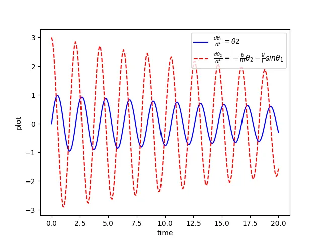
plt.plot(t,theta[:,0],'b-',label=r'$\frac{d\theta_1}{dt}=\theta2$')
#plot of t vs angular velocity
plt.plot(t,theta[:,1],'r--',label=r'$\frac{d\theta_2}{dt}=-\frac{b}{m}\theta_2-\frac{g}{L}sin\theta_1$')
#labelling of plot
plt.ylabel('plot')
plt.xlabel('time')
#giving legend to plot
plt.legend(loc='best')
#command to show the plot
plt.show()


#ct is the count time
ct=1
#for loop fo making animation
for i in angular_displacement:

	#initial condition of string
	x0 = 1
	y0 = 1

	#final condition of the string
	x1=  l-l*math.sin(i)
	y1 = l-l*math.cos(i)

	#file name of the image to be saved in the directory 
	filename = 'animation of pendulam %03d.png' %ct
		
	#plotting of the figure
	plt.figure()
	#plot of the wall having linewidth of 5
	plt.plot([0.5,1.5],[1,1],linewidth=5)
	#ploting of the string
	plt.plot([x0,x1],[y0,y1])
	#plot of the pendulum
	plt.plot(x1,y1,'o',markersize=15)
	#defining the axis of the plot
	plt.axis([-0.5,2.5,-0.5,1.5])
	
	#saveing of the image in the directory
	plt.savefig(filename)

	#increament of the count time
	ct= ct+1

Graph-

Animation link-

https://drive.google.com/file/d/1SSUF8aGmDWGGVJHr__UoKKkECJ9LupFd/view?usp=sharing

results-

The graph of pendulum and the animation is created sucessfully.