Week 5 - Curve fitting

1. What does popt and pcov mean?

Answer:

The curve_fit () function will return the two values; popt and pcov.

The ‘popt’ is an array that represents the optimal values for the parameters to minimize the sum of squared residuals.

The curvefit imported from the scipy module calculate the values of the co-efficient in an equation which is declared inside the function. The values of the co-efficient will be assigned to popt. This can be further used in place of defining parameters while calling the function, which has those coefficients as its parameter.

At the same time, the ‘pcov’ is the 2D array that represents the estimated covariance of ‘popt’. The diagonals provide the variance of the parameter estimate.

2. What does np. array(temperature) do?

Answer:

The NumPy (Numerical python) library contains multidimensional array and matrix data structures. It provides ndarray, a homogeneous n-dimensional array object, with methods to efficiently operate on it. NumPy can be used to perform a wide variety of mathematical operations on arrays. It adds powerful data structures to Python that guarantee efficient calculations with arrays and matrices and it supplies an enormous library of high-level mathematical functions that operate on these arrays and matrices.

np.array (temperature) reads the data of temperature of python list into higher dimensional nparray data which is useful for wide variety of mathematical operations.

3. What does the * in *popt mean?

It is the reference operator used to refer the coefficient present in the popt.

4. Write code to fit a linear and cubic polynomial for the Cp data. Explain if your results are good or bad.?

Detailed explanation:

• Curve_fit function imported from the scipy module is used to determine the true nature of the given curve.
• The read_file () function is defined to read the data from the file which contains the specific heat values for the given temperatures which are separated by comma. So, inside that function the split command is used to split both the values and store them in the two different arrays.
• In the main program the read function was called and then the values are stored in the temperature and cp.
• Popt, pocv = cuve_fit (linear_polynomial, t, cp). This code is given to fetch the co-efficient required for the linear polynomial expression, the curve fit function calculates the value for the co-efficient and stores them in the ‘popt’ and their covariance values are stored in the ‘pcov’.
• fit_cpL = linear_polynomial (np. array(t), *popt). This code is given to call the linear_polynomial function by passing the value of temperature list as the numpy array with *popt which has the values of co-efficient for the other parameters in the function.
• The same steps are repeated for the Cubic_polynomial function also.
  Popt1, pocv1 = cuve_fit (Cubic_polynomial, t, cp), This code is given to fetch the co-efficient required for the Cubic polynomial expression, the curve fit function calculates the value for the co-efficient and stores them in the ‘popt1’ and their covariance values are stored in the ‘pcov1’.
• fit_cpC = Cubic_polynomial (np. array(t), *popt). This code is given to call the Cubic_polynomial function by passing the value of temperature list as the numpy array with *popt which has the values of co-efficient for the other parameters in the function.
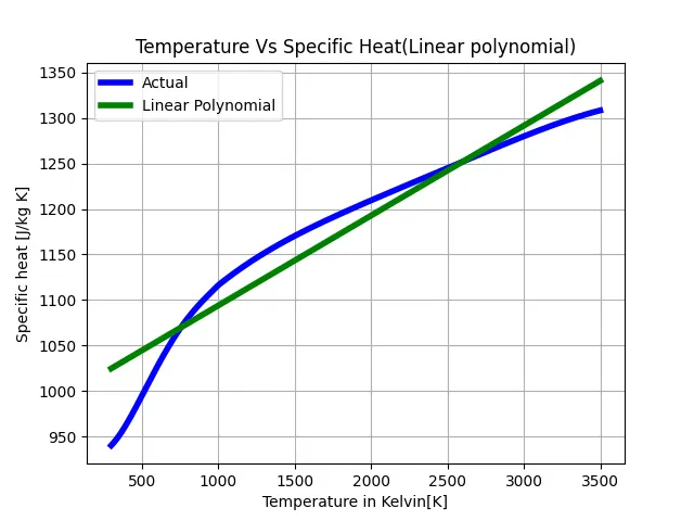
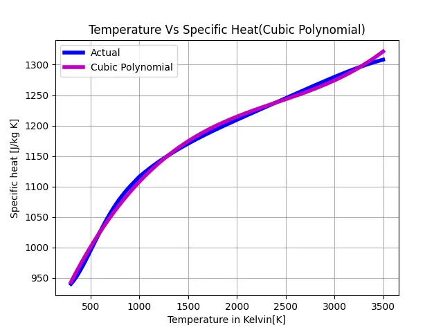
• Then the values stored in the fit_cpL (cp values for linear polynomial function) and fit_cpC (cp values for cubic polynomial function) were plotted along with the temperature values. Plt.savefig (‘Name’) command used to save the plot files.
• Plt.show() command used to show the results of plot.
• For more clarity the plot is made in such a way along with the plot actual value of temperature and cp, So, that it is easy to compare how the curve fit function is performed.

Python Code:

import math
import matplotlib.pyplot as plt
import numpy as np
from scipy.optimize import curve_fit

# Defining the linear equation in function
def linerar_polynomial(t,a,b):
	return a*t+b 
# Defining the cubic polynomial equation in a function
def cubic_polynomial(t,a,b,c,d):
	return a*pow(t,3)+b*pow(t,2)+c*t+d

# Defining function for reading the content in the data file.
def read_file():
	t = [] 							 # Empty array for temperature
	cp =[]  						 # Empty array for Specific heat

	for line in open('data','r'):     # reading the data from file
		values =line.split(',')		  # splitting the data by comma 
		t.append(float(values[0]))    # assigning the values of first line temperature values to t array
		cp.append(float(values[1]))	  # assigning the values of second line cp values to cp array
	return[t,cp]

#main Program to curve fit

t,cp = read_file()  #calling fucnction so that data assigned to the variables

# Calling Linear polynomial function and plotting the curve
popt,pcov = curve_fit(linerar_polynomial,t,cp) # Curve fitting the linear polynomial equation
fit_cpL =linerar_polynomial(np.array(t),*popt) # calling linear polynomial function

# Plotting the temperature vs specific heat curves(For linear equation)
plt.figure('Temperature Vs Specific Heat(Linear Polynomial)')    # Naming the Figure
plt.plot(t,cp,color='b',linewidth = 4)					# Plotting Acutal data	
plt.plot(t,fit_cpL,color ='g',linewidth=4)				# Plotting the Linear polynomial data in green color
plt.xlabel('Temperature in Kelvin[K]')					# Naming the X-axis
plt.ylabel('Specific heat [J/kg K]')  					# Naming the Y-axis
plt.grid()													 # Providing Grid
plt.title('Temperature Vs Specific Heat(Linear polynomial)') # providing Tittle
plt.legend(['Actual','Linear Polynomial'],loc='best')   # creating Legends
plt.savefig('Actual Vs Linear Polynomial')    			#Saving the plot figure

# Calling Cubic polynomial function and plotting the curve

popt1,pcov1 = curve_fit(cubic_polynomial,t,cp) # Curve fitting the cubic polynomial equation
fit_cpC = cubic_polynomial(np.array(t),*popt1) # Calling Cubic polynomial funchtion

# Plotting the temperature vs specific heat curves(For linear equation)
plt.figure('Temperature Vs Specific Heat(Cubic Polynomial)')
plt.plot(t,cp,color='b',linewidth = 4)
plt.plot(t,fit_cpC,color ='m',linewidth=4)
plt.xlabel('Temperature in Kelvin[K]')
plt.ylabel('Specific heat [J/kg K]')
plt.grid()
plt.title('Temperature Vs Specific Heat(Cubic Polynomial)')
plt.legend(['Actual','Cubic Polynomial'],loc='best')
plt.savefig('Actual Vs Cubic Polynomial')
plt.show()

Output & Results:

Conclusion:

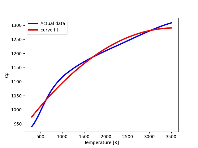
Form the above three plots we can observe that the accuracy of the curve is more increase of order of polynomial means that cubic polynomial plot is more accurate than the quadratic, linear polynomial plots.

First & third plots are generated from above program and 2^nd plot is taken from the example explained in Skill Lync video to show the variation in plots with the increase in order of polynomial.

As analytical observation we can conclude that the order or the degree of equation increases, we get reduce number of errors, so that best curve fit can be obtained.

5. What needs to be done in order to make the curve fit perfect?

Answer: The most common way to fit curves to the data using linear regression is to include polynomial terms, such as squared or cubed predictors.

Typically, you choose the model order by the number of bends you need in your line. Each increase in the exponent produces one more bend in the curved fitted line. It’s very rare to use more than a cubic term.

To achieve the proper curve_fit, the right order or the degree of the curve to be selected. By doing so we can achieve much better curve than the cubic_polynomial curve

6. Show empirically as to how well your curve has been fit.

Answer: From the output of above program we can observe that the order or the degree of equation increases, we get reduce number of errors, so that best curve fit can be obtained.