Week 5 - Curve fitting
curve fit:
AIM:
To write a python code to obtain a best fitting curve.
THEORY:
Curve fitting is the process of constructing a curve, or mathematical function, that has the best fit to a series of data points, possibly subject to constraints. Fitted curves can be used as an aid for data visualization, to infer values of a function where no data are available, and to summarize the relationships among two or more variables.
The method of least squares is a widely used method of fitting curve for a given data. It is the most popular method used to determine the position of the trend line of a given time series. The trend line is technically called the best fit.The problem of finding the curve that best fits a number of data points. The philosophical interest lies in justifying any particular trade-off of simplicity, accuracy, and boldness, that may commend itself. The problem of induction can be represented graphically as a curve-fitting problem.
procedure:
first open a new script and save it as curve.py (.py extension is must)
then for linear, cubic and spiltwise method individual code has to be write.
the code are shown below.
then finally the rms value has to obtain for this write a code.
now build the code we obtain a plot with the actual data and the curve fit.
the same has to done with sligth modification to obtain the curve fit and the rms value.
python code:
# for linear curve fit:

import math as m
import numpy as np
import matplotlib.pyplot as plt
from scipy.optimize import curve_fit

def read_file():
	temp=[]
	cp=[]
	for line in open('curve','r'):
		value=line.split(',')
		temp.append(float(value[0]))
		cp.append(float(value[1]))
	return[temp,cp]


def func(t,a,b):
	return a*t+b

temperature,cp= read_file()

popt,pcov=curve_fit(func,temperature,cp)
predicted_cp= func(np.array(temperature),*popt)


plt.plot(temperature,cp,color='blue',linewidth='3')
plt.plot(temperature,predicted_cp,color='red',linewidth='3')
plt.legend(['actual curve','curvefit'])
plt.xlabel('temperature[k]')
plt.ylabel('specific heat[kj/(kg*k)]')
plt.show()

a=pow((cp-predicted_cp),2)
sse= np.sum(a)

b=np.mean(cp)
c=pow((predicted_cp-b),2)

ssr= np.sum(c)
sst=sse+ssr

r_square=ssr/sst
print(r_square)


#for cubic curve fit:

import math as m
import numpy as np
import matplotlib.pyplot as plt
from scipy.optimize import curve_fit

def read_file():
	temp=[]
	cp=[]
	for line in open('curve','r'):
		value=line.split(',')
		temp.append(float(value[0]))
		cp.append(float(value[1]))
	return[temp,cp]


def func(t,a,b,c,d):
	return a*pow(t,3)+b*pow(t,2)+c*t+d

temperature,cp= read_file()

popt,pcov=curve_fit(func,temperature,cp)
predicted_cp= func(np.array(temperature),*popt)


plt.plot(temperature,cp,color='blue',linewidth='3')
plt.plot(temperature,predicted_cp,color='red',linewidth='3')
plt.legend(['actual curve','curvefit'])
plt.xlabel('temperature[k]')
plt.ylabel('specific heat[kj/(kg*k)]')
plt.show()

a=pow((cp-predicted_cp),2)
sse= np.sum(a)

b=np.mean(cp)
c=pow((predicted_cp-b),2)

ssr= np.sum(c)
sst=sse+ssr

r_square=ssr/sst
print(r_square)


#for splitwise method:
import math as m
import numpy as np
import matplotlib.pyplot as plt
from scipy.optimize import curve_fit

def read_file():
	temp=[]
	cp=[]
	for line in open('curve','r'):
		value=line.split(',')
		temp.append(float(value[0]))
		cp.append(float(value[1]))
	return[temp,cp]


def func(t,a,b,c,d):
	return a*pow(t,3)+b*pow(t,2)+c*t+d

temperature,cp= read_file()
temperature_1=np.array(temperature[0:800])
cp_1=np.array(cp[0:800])
popt,pcov=curve_fit(func,temperature_1,cp_1)
predicted_cp_1= func(np.array(temperature_1),*popt)


temperature_2=np.array(temperature[801:1600])
cp_2=np.array(cp[801:1600])
popt,pcov=curve_fit(func,temperature_2,cp_2)
predicted_cp_2= func(np.array(temperature_2),*popt)

temperature_3=np.array(temperature[1601:2400])
cp_3=np.array(cp[1601:2400])
popt,pcov=curve_fit(func,temperature_3,cp_3)
predicted_cp_3= func(np.array(temperature_3),*popt)

temperature_4=np.array(temperature[2401:3200])
cp_4=np.array(cp[2401:3200])
popt,pcov=curve_fit(func,temperature_4,cp_4)
predicted_cp_4= func(np.array(temperature_4),*popt)


plt.plot(temperature,cp,color='blue',linewidth='3')
plt.plot(temperature_1,predicted_cp_1,color='green',linewidth='3')
plt.plot(temperature_2,predicted_cp_2,color='yellow',linewidth='3')
plt.plot(temperature_3,predicted_cp_3,color='green',linewidth='3')
plt.plot(temperature_4,predicted_cp_4,color='yellow',linewidth='3')
plt.legend(['actual curve','curvefit'])
plt.xlabel('temperature[k]')
plt.ylabel('specific heat[kj/(kg*k)]')
plt.show()

#root mean square value:

a=pow((cp_1-predicted_cp_1),2)
sse= np.sum(a)

b=np.mean(cp_1)
c=pow((predicted_cp_1-b),2)

ssr= np.sum(c)
sst=sse+ssr

r_square_1=ssr/sst
print(r_square_1)


a=pow((cp_2-predicted_cp_2),2)
sse= np.sum(a)

b=np.mean(cp_2)
c=pow((predicted_cp_2-b),2)

ssr= np.sum(c)
sst=sse+ssr

r_square_2=ssr/sst
print(r_square_2)

a=pow((cp_3-predicted_cp_3),2)
sse= np.sum(a)

b=np.mean(cp_3)
c=pow((predicted_cp_3-b),2)

ssr= np.sum(c)
sst=sse+ssr

r_square_3=ssr/sst
print(r_square_3)

a=pow((cp_4-predicted_cp_4),2)
sse= np.sum(a)

b=np.mean(cp_4)
c=pow((predicted_cp_4-b),2)

ssr= np.sum(c)
sst=sse+ssr

r_square=ssr/sst
print(r_square)
results:
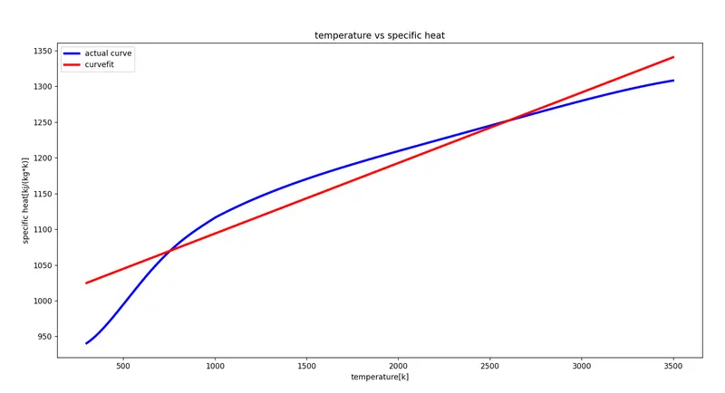
for linear curve fit:
plot:
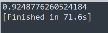
rms value:
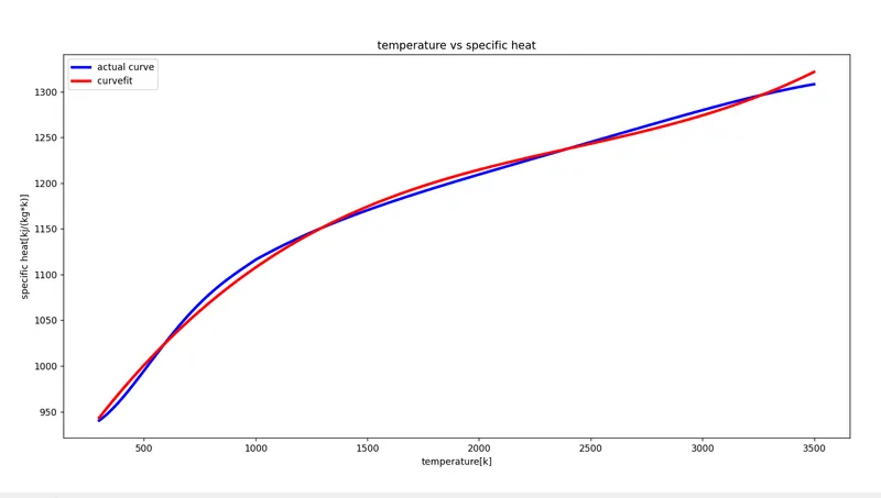
for cubic curve fit:
plot:
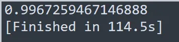
rms value for cubic:
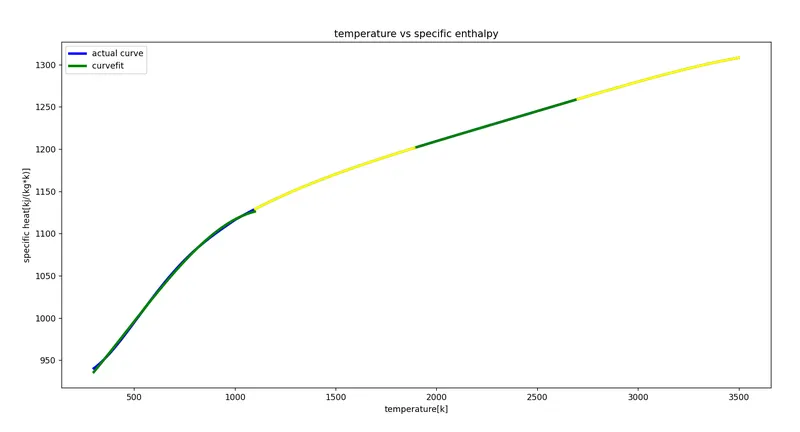
splitwise method:
plot:
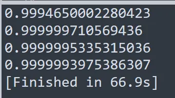
rms for splitwise method:
conclusion:
- hence the curve fit is done for linear, cubic and splitwise method.
- and plotted the actual curve vs curve for the linear, cubic and splitwise method.
- then the root mean square value of the linear , cubic and splitwise has been calculated.
----------------------------------thank you----------------------------