Week 5 - Curve fitting

Aim:

write a python code to fit a linear and cubic polynomial for the given Cp data.

OBJECTIVES:

• curve fit the Cp data in linear and cubic polynomial .
• To plotting the linear and cubic fit curves.

Theory:

for a given a series of data points, the process of constructing a curve having the best fit subjected to given constraints is called as curve fitting.

interpolations techniques can be used to fit the curve exactly to the data.

1. What does popt and pcov mean?

popt: It gives optimal coefficient values in an array with the parameters so that the sum of the square of the residuals of the given data is minimized

pcov:It is the estimated covariance of popt which is of dimensions n+1/n+1 in matrix form

2. What does np.array(temperature) do?

np.array is used to Store values in the array of the curve fitting function. 

3. What does the * in *popt mean?

* in *popt: It stores the values (in the array popt) of the parameters(a,b,c).

4. Write code to fit a linear and cubic polynomial for the Cp data. Explain if your results are good or bad. 

Code:

import math
import numpy as np
import matplotlib.pyplot as plt
from scipy.optimize import curve_fit

def read_file():
	temperature = []
	cp = []
	for line in open('data','r'):
		value = line.split(',')
		temperature.append(float(value[0]))
		cp.append(float(value[1]))
	return [temperature, cp]
		#pass

# curve fir function (linear polynomial)
def func(t,a,b):
	return a*t+b

temperature, cp = read_file()
#print(temperature)

popt,pcov = curve_fit(func, temperature,cp)
fit_cp = func(np.array(temperature), *popt)

T,cp = read_file()

plt.plot(T,cp)
plt.plot(temperature,fit_cp)
plt.xlabel('temperature')
plt.ylabel('specific heat at constant pressure Cp')
plt.title('Linear curve fit data', fontweight = "bold")
plt.show()



# curve fit function (cubic polynomial)
def func(t,a,b,c,d):
	return a*pow(t,3)+b*pow(t,2)+ c*t+d
temperature, cp = read_file()
#print(temperature)

popt,pcov = curve_fit(func, temperature,cp)
fit_cp = func(np.array(temperature), *popt)

T,cp = read_file()
plt.plot(T,cp)
plt.plot(temperature,fit_cp)
plt.xlabel('temperature')
plt.ylabel('specific heat at constant pressure Cp')
plt.title('Cubic polynomial curve fit data', fontweight = "bold")
plt.show()

 Results and Discussion:

The above code will yield two plots as shown below, Figure 1 is using Linear polynomial function, while Figure 2 uses Cubic Polynomial function.

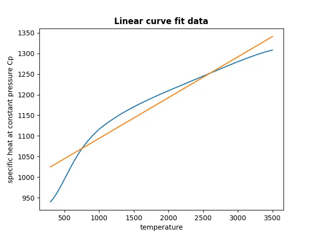
                                                              Figure 1

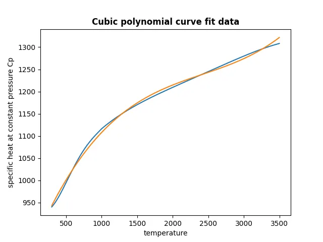
                                                             Figure 2

It can be seen from Figure 1 that the Linear polynomial function does not match the points as described by the data, Therefore this is not a good fit for our given data. while the cubicpolynomial function matches closer to the given data. 

5. What needs to be done in order to make the curve fit perfect?

Increasing the order of the polynomial to make the curve fit perfect as shown above.