Week 3 - Solving second order ODEs

Aim/Objective:

To write a program to solve equation of motion of a simple pendulum with damping

Theory:

A second order differential equation consists of a derivative of an order 2 (of a function ) and no other higher order derivative. It includes terms like Y”, d²y/dx² etc.

Simple Pendulum:

A simple pendulum is a mechanical system having an oscillatory motion, consisting of a mass ’m’ suspended with the an inextensible string of length L. The motion occurs in a vertical plane and is driven by a gravitational force.

An ODE is a differential equation that has one or more functions of both independent variable and derivatives of these functions.

The equation of motion of a simple pendulum is represented by an ordinary differential equation.

In case a simple pendulum is tilted at an initial angle and released, the pendulum will execute a simple harmonic motion by swinging back and forth.

This is explained by Newton’s second law and its studies.

Governing Equation :

The primary Differential equation to be solved is `{d^2θ}/(d t^2) + b/m (dθ)/(d t) + g/L sin θ = 0`

substitute `theta = theta_1`

`(d theta )/(dt) = (d theta_1)/(dt)`

`(d theta_1)/(dt)= theta_2`

`{d^2θ}/(d t^2) = (d^2θ_1)/(d t^2) = d/dt((dθ_1)/(d t))= d/dt(θ_2)`

the governing equation now becomes

`{dθ_2 }/(d t) + b/mθ_2+g/L sintheta_1=0`

`implies (d theta_2)/(dt) =- b/mθ_2+g/L sintheta_1`

This is a second order differential equation

Solution Procedure :

Python Code:

#Step 1 
import numpy as np
from scipy.integrate import odeint
import math
import matplotlib.pyplot as plt
#Step 2
def function(theta,t,b,g,l,m):
	theta1 = theta[0]
	theta2 = theta[1]
	dtheta1_dt = theta2
	dtheta2_dt = -(b/m)*theta2-(g/l)*math.sin(theta1)
	dtheta_dt = [dtheta1_dt,dtheta2_dt]
	return dtheta_dt
#Step 3
b= 0.05
g = 9.81
l=1
m=1

theta_0 = [0,3]

t= np.linspace(0,20,150)
#Step 4
theta = odeint(function,theta_0,t,args = (b,g,l,m))
#Step 5
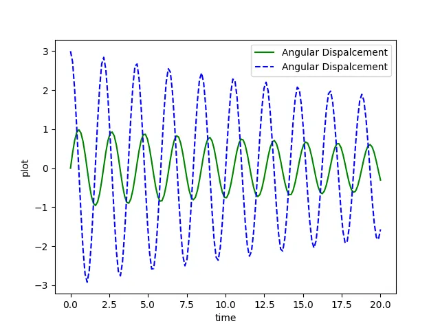
plt.plot(t,theta[:,0],'g-',label = 'Angular Dispalcement')
plt.plot(t,theta[:,1],'b--',label = 'Angular Dispalcement')
plt.ylabel('plot')
plt.xlabel('time')
plt.legend(loc='best')
plt.show()


#Step 6
 
ct = 1
x0 = 0
y0 = 0




for i in theta[:,0]:
	x1 = x0 + (l*math.sin(i))
	y1 = y0 - (l*math.cos(i))
	filename = str(ct) + '.png'
	ct = ct + 1


	plt.figure()
	plt.plot([-1,1],[0,0],'black')
	plt.plot([x0,x1],[y0,y1],'red')
	plt.plot(x1,y1,'o', markersize = '20')
	plt.xlim([-1.5,1.5])
	plt.ylim([-1.5,1.0])
	plt.title('Simple Pendulum')
	plt.savefig(filename)

Step wise explanation of the code.

• Step 1: Importing requsite libraries
  • Scipy.integrate containes the odeint library that is used for integration.
• Step 2 : Function Definition
  • The function is defined to compute the ODE's mentioned above.
• Step 3 : Inputing variables (Defining the inputs)
  • In this step we define the damping coefficient, value of acceleration due to gravity, length of the pendulum ,etc
• Step 4 : Solving the Problem.
  • The function previously defined is called with the odeint library to solve the function (governing equation in the simplified form)
• Step 5 : Ploting the graphs
  • Plotting the solution of the 2 ode's obtained program using mathplotlib module
• Step 6 : Creating and Animating the plot
  • Creating images for animation and Saving the images obtained.

Errors Obtained.

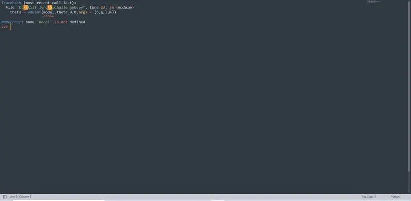
• Improper use of function: solved by observing that the function definition is not included in the Step 4
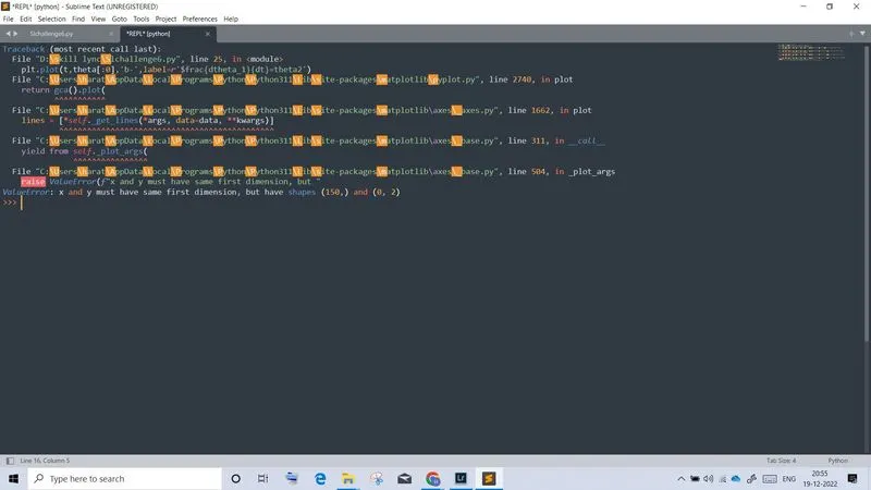
• Improper usage of syntax in Step 5: Solved this by observing the syntax of plotting.

Screenshots showing errors thrown in command window.

Output:

Animation video