Week 2 Air standard Cycle

Aim :

To write a Python program that solves an otto cycle and obtain Plots and Thermal efficiency

Equations used:

Swept volume (m³): `V_s=π/4×d^2×L`

Clearance volume (m³): `V_c=V_s/(r-1)`

Volume @ BDC (m³): `V_1=V_4=V_s+V_c`

Volume @ TDC (m³): `V_2=V_3=V_c`

PV Relations (m³) : `P_1×V_1^γ=P_2×V_2^γ`

PVT Relations (m³): `(P_1×V_1)/T_1 =(P_2×V_2)/T_2`

Instantaneous Volume (m³) : `V_θ=V_c×(1+(r-1)/2)×{1+R-Cosθ-(R^2-sin^2⁡θ )^(1/2) }`

{where `R=2×L_cr/L`}

Instantaneous Pressure (MPa): `P_θ×V_θ^γ=P_2×V_2^γ`

Thermal Efficiency : `1-(T_4-T_1)/(T_3-T_2 )`

Where

• D = Bore Diameter
• L = Stroke
• L_cr = Connecting rod Length
• r= Compression Ratio

Objective:

To solve otto cycle.

Obtain PV values during intake, compression, expansion, and exit stroke and plot the P-V graph

Calculate the efficiency of the otto-cycle

Solution Procedure :

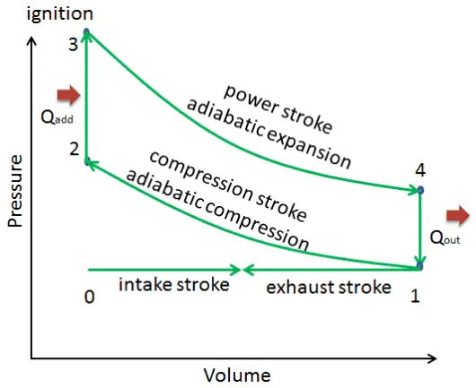
An otto cycle is made up of four reversible processes:

1-2 isentropic compression

2-3 constant volume heat addition

3-4 isentropic expansion

4-1 constant volume heat rejection

Air is compressed in process 1-2 reversibly and adiabatically. Heat is then added to air reversibly at constant volume in process 2-3. Work is done by air in expanding reversibly and adiabatically in process 3-4. Heat is then rejected by air reversibly at constant volume in process 4-1, and the system comes back to its initial state

Code :

import math
import matplotlib.pyplot as plt
import numpy as np

def engine_kinematics(bore, stroke, con_rod, cr, start_crank, end_crank):
	a = stroke/2
	R = con_rod/a
	v_s = (math.pi/4)*pow(bore,2)*stroke
	v_c = v_s/(cr-1)

	sc = math.radians(start_crank)
	ec = math.radians(end_crank)

	theta = np.linspace(sc,ec,50)

	v=[]

	for i in range(0,50):

		Theta = theta[i]

		term1 = 0.5*(cr-1)
		term2 = R + 1- math.cos(Theta)
		term3 = pow(R,2) - pow(math.sin(Theta),2)
		term3 = pow(term3,0.5)

		v.append((1 + term1*(term2-term3))*v_c)
		pass


	return v
	pass


# input variables
gamma = 1.4
T3 = 2000

p1 = 101325
T1 = 350


bore=0.12
stroke = 0.1
connecting_rod = 0.15
c_r = 10

# swept volume and clearance volume
v_swept = (math.pi/4)*pow(bore,2)*stroke
V_clearance = v_swept/(c_r-1)
v1 = v_swept+V_clearance
v2 = V_clearance

#calculation of p2 and T2
p2 = p1*pow(c_r,gamma)

T2= p2*v2*T1/(p1*v1)

V_comp = engine_kinematics(bore, stroke, connecting_rod, c_r, 180, 0)
C_const = p1*pow(v1,gamma)
P_comp = []

for V in V_comp:
	P_comp.append(C_const/pow(V,gamma))
	pass

p3 = p2*(T2/T3)
v3 = v2

V_expp = engine_kinematics(bore, stroke, connecting_rod, c_r, 0, 180)
C_const = p3*pow(v3,gamma)
P_expp = []

print(V_expp)

for V in V_expp:
	P_expp.append(C_const/pow(V,gamma))
	pass
print(P_expp)
v4 = v1
p4 = p3*pow(v3,gamma)/pow(v4,gamma)

plt.plot([v1,v2,v3,v4,v1],[p1,p2,p3,p4,p1])
plt.xlabel('volume(m^3)')
plt.ylabel('Pressure(Pa)')
plt.title('p-V diagram of an Otto Cycle', fontweight = "bold")
plt.grid()
plt.show()

plt.plot(V_comp,P_comp)
plt.plot(V_expp,P_expp)
plt.plot([v2,v3],[p2,p3])
plt.plot([v4,v1],[p4,p1])
plt.xlabel('volume(m^3)')
plt.ylabel('Pressure(Pa)')
plt.title('P-V diagram of an Otto Cycle', fontweight = "bold")
plt.grid()
plt.show()

T4 = (p4*v4*T3)/(p3*v3)

Thermal_eff = (1-((T4-T1)/(T3-T2)))

print(Thermal_eff)

Results :

The PV Diagram of an otto cycle is as shown below

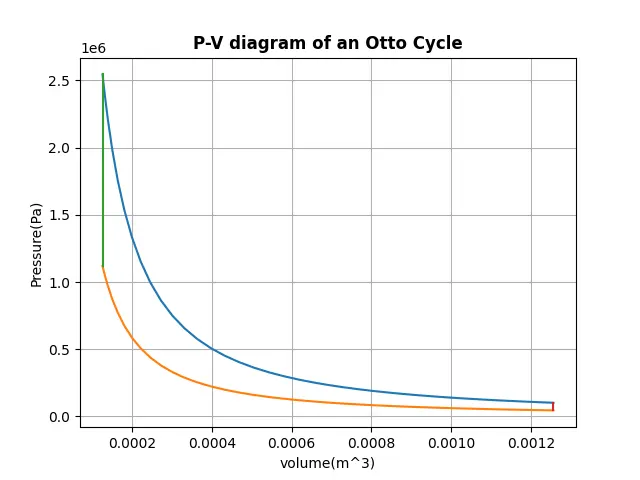
The thermal efficiency of the otto cycle obtained is 60.189%