Week 5 - Curve fitting

objective

1. What does popt and pcov mean? 

2. What does np.array(temperature) do?

3. What does the * in *popt mean?

4. Write code to fit a linear and cubic polynomial for the Cp data. Explain if your results are good or bad. 

5. What needs to be done in order to make the curve fit perfect?

6. Show empirically as to how well your curve has been fit.

ans

1.popt and pcov

The popt argument are the best-fit paramters 

The pcov variable contains the covariance matrix, which indicates the uncertainties and correlations between parameters. This is mostly useful when the data has uncertainties.

2. np.array([temp])

this create a numpy array of tepmrature

A numpy array is a grid of values, all of the same type, and is indexed by a tuple of nonnegative integers. 

3. * in *popt

The * notation will expand a list of values into the arguments of the function. This is useful if your function has more than one or two parameters. 

4.

linear fit

#linear curve fit
import numpy as np
from scipy.optimize import curve_fit
import matplotlib.pyplot as plt 

#function define for curve fit
def func(t,b,c):
    return(b*t+c)

#function to read file
def read_file():
    temp=[];
    cp=[];
    for line in open('data','r'):
        value=line.split(',');#split the data data
        temp.append(float(value[0]));#conver string to float
        cp.append(float(value[1]))
    return [temp,cp]
temp,cp=read_file();
popt,pcov=curve_fit(func,temp,cp);#curve fit coeffieceint calculation
fit_cp=func(np.array(temp),*popt);#new cp for new curve fit coeffeceint


#plots
plt.plot(temp,cp);
plt.plot(temp,fit_cp)
plt.legend(['actual data plot','curve fit plot'])
plt.xlabel('temp in k')
plt.ylabel('cp in j/kg*k')

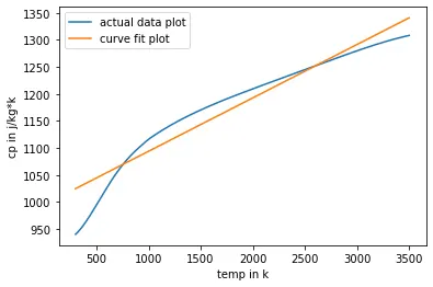
linear curve fit

cubic curve fit

import numpy as np
from scipy.optimize import curve_fit
import matplotlib.pyplot as plt 

#function define for curve fit
def func(t,a,b,c,d):
    return(a*t**3+b*t**2+c*t+d)
#function to read file
def read_file():
    temp=[];
    cp=[];
    for line in open('data','r'):
        value=line.split(',');#split the data data
        temp.append(float(value[0]));#conver string to float
        cp.append(float(value[1]))
    return [temp,cp]
temp,cp=read_file();
popt,pcov=curve_fit(func,temp,cp);#curve fit coeffieceint calculation
fit_cp=func(np.array(temp),*popt);#new cp for new curve fit coeffeceint


#plots
plt.plot(temp,cp);
plt.plot(temp,fit_cp)
plt.legend(['actual data','curve fit'])
plt.xlabel('temp in k')
plt.ylabel('cp in j/kg*k')

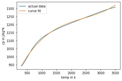
cubic curve fit

5. improve curve fitting

to improve the curve fitting needs to do higer order curve fitting then curve fitting will be more accurate but its deficult task but by spliting temp in small section and the curve fitting gives best result

5.empraical solution of curvefit

for linear curve fit

Goodness of fit:
SSE: 2.163e+06
R-square: 0.9249
Adjusted R-square: 0.9249
RMSE: 26.01

for cubic curve fit

Goodness of fit:
SSE: 9.427e+04
R-square: 0.9967
Adjusted R-square: 0.9967
RMSE: 5.431