Week 5 - Curve fitting

1. What does popt and pcov mean?

The curve_fit function returns two items, which is popt and pcov.

popt - The popt arguments are the best-fit parameters. It is an array of optimal values for the parameters which minimize the sum of squares of residuals.

pcov - The pcov variable contains the covariance matrix, which indicates the uncertainties and correlations between parameters. This is most useful when the data has uncertainties.

2. What does np.array(temperature) do?

The np.array(temperature) converts the python list into a numpy array because some mathematical operations cannot be performed in python lists but we can do it in numpy array.

3. What does the * in *popt mean?

* is used to pass a variable number of arguments to a function. Here, it is used to pass the values stored in the array popt.

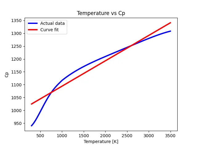
4. Write code to fit a linear and cubic polynomial for the Cp data. Explain if your results are good or bad.

Linear polynomial:

from turtle import color
import numpy as np
import matplotlib.pyplot as plt
from scipy.optimize import curve_fit

#curve fit function
def fun(t,a,b):
    return a*t+b  #linear polynomial

#reading thermodynamic data file
def read_file():
    temperature=[]
    cp=[]
    for line in open('data','r'):
        values = line.split(',')  
        temperature.append(float(values[0]))  
        cp.append(float(values[1]))

    return [temperature,cp]

#main program 
temperature,cp = read_file()
popt,pcov = curve_fit(fun,temperature,cp) 
fit_cp = fun(np.array(temperature),*popt)

plt.plot(temperature,cp,color='blue',linewidth=3)
plt.plot(temperature,fit_cp,color='red',linewidth=3)
plt.legend(['Actual data','Curve fit'])
plt.xlabel('Temperature [K]')
plt.ylabel('Cp')
plt.title('Temperature vs Cp')
plt.show()

Output:

Cubic polynomial:

from turtle import color
import numpy as np
import matplotlib.pyplot as plt
from scipy.optimize import curve_fit

#curve fit function
def fun(t,a,b,c,d):
    return a*pow(t,3)+b*pow(t,2)+c*t+d  #cubic polynomial

#reading thermodynamic data file
def read_file():
    temperature=[]
    cp=[]
    for line in open('data','r'):
        values = line.split(',')
        temperature.append(float(values[0]))  
        cp.append(float(values[1]))

    return [temperature,cp]

#main program 
temperature,cp = read_file()
popt,pcov = curve_fit(fun,temperature,cp) 
fit_cp = fun(np.array(temperature),*popt)

plt.plot(temperature,cp,color='blue',linewidth=3)
plt.plot(temperature,fit_cp,color='red',linewidth=3)
plt.legend(['Actual data','Curve fit'])
plt.xlabel('Temperature [K]')
plt.ylabel('Cp')
plt.title('Temperature vs Cp')
plt.show()

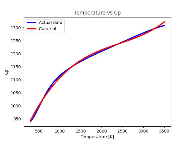
Output:

Results:

By comparing the output from both the linear and cubic polynomials, we can definitely say that the cubic polynomial fit is the best as it traces the actual data very close.

Code explanation:

1. import
   • numpy is imported as we are performing some mathematical operations
   • matplotlib is used for plotting the data
   • scipy is used for the curve fit function
2. Next, we are defining the function for the curve fit as a linear or cubic polynomial.
3. read_file()
   • After that, we are defining a function called read_file() to read the thermodynamic data file from the notepad.
   • Next we use line.split(',') command to split the values in the notepad.
   • Next, we use append command to store the values of temperature and cp in separate variables, temperature and cp.
4. main program
   • function call for read_file to get the values of temperature and cp
   • Next, we perform the curve fit operation by passing the curve fit function and temperature and cp values.
   • After getting the required values, popt values are used for fitting the curve.
5. Next, we plot the actual data and the curve fit data separately.

5. What needs to be done in order to make the curve fit perfect?

Perfect curve fit means that the fitted curve should exactly trace the actual data. By doing the comparison between linear and cubic polynomials, we found that the cubic fit was best. So, in order to make the curve fit perfectly, we have to increase the order of the polynomial.

6. Show empirically as to how well your curve has been fit.

From observation, it is seen that the cubic fit almost traced the actual data with some tolerances compared to linear fit.

The below data shows how the curve fit values compare with the actual data for cubic polynomial.

Cp = [940.3659512022349, 940.53912184539, 940.7138187558996, 940.8900327242061, 941.0677545614627, 941.2469750995348, 941.4276851909997, 941.609875709146, 941.7935375479744,....1307.8230899530042, 1307.8659787751492, 1307.9087882322265, 1307.9515181753247, 1307.9941684553978, 1308.0367389232608, 1308.0792294295902, 1308.121639824924, 1308.1639699596617]

Fit cp = [ 943.34732591 943.65736782 943.96716791 ... 1321.36153246 1321.4827291
1321.60404955]