Week 5 - Curve fitting
1) POPT - An array of the optimal coefficient values for the parameters which minimizes the sum of squares of the remaining values.
PCOV - It is the secondary or the returned parameter covariance matrix of the estimated POPT based on a scaling sigma by a constant factor. The diagonals provide the variance of the parameter estimate.
2) np.array converts the temperature data list to a numpy array since operations like pow are allowed on numpy arrays.
3) The '*' in '*OPT' represents refers to the values stored in POPT array.
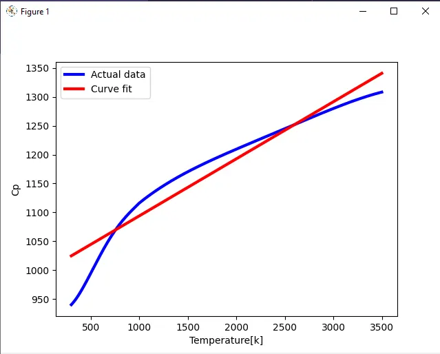
4) Write code to fit a linear and cubic polynomial for the Cp data. Explain if your results are good or bad.
--> LINEAR POLYNOMIAL
Code:
import numpy as np
import matplotlib.pyplot as plt
from scipy.optimize import curve_fit
# Curve fit function
def func(t, a, b, c):
return a*t + b
# Return thermodynamic data file
def read_file():
temperature = []
cp = []
for line in open('data','r'):
values = line.split(',')
temperature.append(float(values[0]))
cp.append(float(values[1]))
return [temperature,cp]
#Main program
temperature, cp = read_file()
popt, pcov = curve_fit(func, temperature, cp) #popt are the coeffecients namely a,b,c
fit_cp = func(np.array(temperature), *popt)
plt.plot(temperature, cp,color="blue",linewidth=3)
plt.plot(temperature, fit_cp,color="red",linewidth=3)
plt.legend(['Actual data','Curve fit'])
plt.xlabel('Temperature[k]')
plt.ylabel('Cp')
plt.show()
Output:
CUBIC POLYNOMIAL
Code:
import numpy as np
import matplotlib.pyplot as plt
from scipy.optimize import curve_fit
# Curve fit function
def func(t, a, b, c, d):
return a*pow(t,3) + b*pow(t,2) + c*t + d
# Return thermodynamic data file
def read_file():
temperature = []
cp = []
for line in open('data','r'):
values = line.split(',')
temperature.append(float(values[0]))
cp.append(float(values[1]))
return [temperature,cp]
#Main program
temperature, cp = read_file()
popt, pcov = curve_fit(func, temperature, cp) #popt are the coeffecients namely a,b,c
fit_cp = func(np.array(temperature), *popt)
plt.plot(temperature, cp,color="green",linewidth=3)
plt.plot(temperature, fit_cp,color="black",linewidth=3)
plt.legend(['Actual data','Curve fit'])
plt.xlabel('Temperature[k]')
plt.ylabel('Cp')
plt.show()
Output:
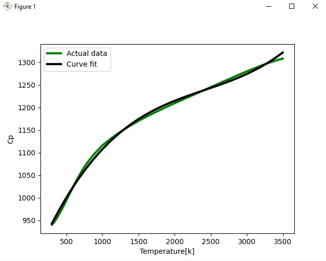
With respect to the plotted graphs, we can come to a conclusion that the results are good as the cubic fit has a better curve fit than the linear fit.
5) What needs to be done in order to make the curve fit perfect?
i) As the degree of the curve increases, the curve gets better.
ii) The 4th degree polynomial has a better curve fit compared to the cubic polynomial curve.
iii) But, further inceasing the degree of the polynomial would make the curve more complex and would also consume time. Therefore, the 4th degree polynomial curve is considered as the best fit curve.
6) Show empirically as to how well your curve has been fit.
As per the observation with respect to the plotted curves, a cubic predicted curve has been almost fit into original data curve with some tolerance compared to linear predicted curve. If curve fit overlapped to original data with some defined tolerances, it is called best fit. The perfect fit is always a best fit, but the best fit is not a perfect fit.