Week 3 - Solving second order ODEs

Code:

import numpy as np
from scipy.integrate import odeint
import matplotlib.pyplot as plt
import math
from PIL import Image
import glob
#function that returns dz/dt
def model(theta,t,b,g,l,m):
	theta1 = theta[0]
	theta2 = theta[1]
	dtheta1_dt = theta2
	dtheta2_dt = -(b/m)*theta2 - (g/l)*math.sin(theta1)
	dtheta_dt = [dtheta1_dt,dtheta2_dt]
	return dtheta_dt
b = 0.05
g = 9.81
l = 1
m = 0.5
#initial condition
theta_0 = [0,3]
#time points
t = np.linspace(0,15,300)
#solve ODE
theta = odeint(model,theta_0,t,args = (b,g,l,m))
#print(theta)
#plot results
plt.plot(t,theta[:,0],'b-', label = r'$frac {dtheta_1}{dt}=theta2$')
plt.plot(t,theta[:,1],'r--',label = r'$frac{dtheta2}{dt}= -frac{b}{m}theta_2-frac{g}{l}sintheta_1$')
plt.ylabel('plot')
plt.xlabel('time')
plt.legend(loc = 'best')
#plt.savefig('Graph_disvelo')
plt.show()
#plotting simple pendulum on graph at each angle.
x = theta[0,1]
y=theta[:,0]
ct=1
for ang in y :
	x1=0;y1=0
	x2=l*math.sin(ang)
	y2=-l*math.cos(ang) 
	plt.figure()
	plt.plot([-2.0,2.0],[0,0],'y',linewidth=5)
	plt.plot([x1,x2],[y1,y2],linewidth=3)
	plt.plot(x2,y2,'o',markersize=20,markerfacecolor='w')
	plt.plot(x1,y1,'o',markersize=6,markerfacecolor='r')
	plt.xlim([-2.0,2.0])
	plt.ylim([-2.0,0.5])
	filename = 'test%05d.png'%ct
	plt.savefig(filename)
	ct=ct+1
	#creating 'gif' from the images saved
	frames = []
	imgs = glob.glob("*.png")
	for i in imgs:
		new_frame = Image.open(i)
		frames.append(new_frame)
	# Save into a GIF file that loops forever
	frames[0].save('png_to_gif.gif', format='GIF',
		append_images=frames[1:],
		save_all=True,
		duration=60, loop=0)

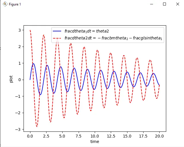
Results: The graph below shows the variation of Angular displacement and velocity of pendulum w.r.t time.

Blue line—Displacement curve.

Redline—Velocity curve.

Youtube link for an animation of the pendulum :

https://www.youtube.com/watch?v=CM9E4l9-wbQ&ab_channel=AbraarAhmad