Week 5 - Curve fitting

Curve Fitting

What is Curve Fitting ?
Curve fitting is the process of constructing a curve, or mathematical functions, which possess the closest proximity to the real series of data. By curve fitting, we can mathematically construct the functional relationship between the observed dataset and parameter values, etc. It is highly effective in the mathematical modeling of some natural processes.

Question 1.

What does popt and pcov mean? (Watch the video to get some context)

Answer :-

• Popt-It is an array.This will be our coefficients in the program.It represents the unknowns
  in the function defined in the program so later it will be the output as it curve fit function
  calculates it.Or in other words optimal values for the parameters so that the sum of the
  squared error is minimized.
• pcov-The estimated covariance of popt. The diagonals provide the variance of the
  parameter estimate.

Question 2.

What does np.array(temperature) do?

Answer :-

• np.array(temperature) stores the values of temperature in the form of array and passes
  it to numpy function.

Question 3.

What does the * in *popt mean?

Answer :-

• It stores the values of unknown variables in popt array.

Question 4.

Write code to fit a linear and cubic polynomial for the Cp data. Explain if your results
are good or bad.

Answer :-

PYTHON CODE :

"""
Program for curve fitting of linear polynomial
"""

import math
import matplotlib.pyplot as plt
import numpy as np
from scipy.optimize import curve_fit

# curve fit funtion
# linear funtion
def function_0(t,a,b):
return a*t + t

# cubic funtion
def function_1(t,a,b,c,d):
return a*pow(t,3) + b*pow(t,2) + c*t + d

# reading thermodinamic data files
def read_file():
tempreature = []
cp = []
for line in open('data','r'):
value = line.split(',')
tempreature.append(float(value[0]))
cp.append(float(value[1]))
return [tempreature,cp]

# main program
#linear curve fitting
tempreature,cp = read_file()

popt,pcov = curve_fit(function_0,tempreature,cp)
fit_cp_l = function_0(np.array(tempreature),*popt)
plt.figure(1)
plt.plot(tempreature,cp,color='red',linewidth=2)
plt.plot(tempreature,fit_cp_l,color='yellow',linewidth=2)
plt.legend(['Actual data','curve fit'])
plt.xlabel('tempreature(k)')
plt.ylabel('cp')
plt.title('linear curve fitting')
plt.show()

#cubic curve fitting
popt,pcov = curve_fit(function_1,tempreature,cp)
fit_cp_c = function_1(np.array(tempreature),*popt)
plt.figure(2)
plt.plot(tempreature,cp,color='red',linewidth=2)
plt.plot(tempreature,fit_cp_c,color='yellow',linewidth=2)
plt.legend(['Actual data','curve fit'])
plt.xlabel('tempreature(k)')
plt.ylabel('cp')
plt.title('cubic curve fitting')
plt.show()

s = np.sum(cp)
l = np.size(cp)
m = s/l
print('mean of all cp:',m)
print('')

# For Linear curve fit
linear_ssr =0
linear_sse =0
for i in range(l):
linear_error = abs((np.sum((cp[i] - fit_cp_l[i]))))
linear_sse = linear_sse + pow(linear_error,2)
linear_ssr = linear_ssr + np.sum(pow((fit_cp_l[1] - m),2))
linear_sst = linear_sse + linear_ssr
print('linear_sst:',linear_sst)
linear_R2 = linear_ssr/linear_sst
print('linear_R2:',linear_R2)
linear_rmse = pow((linear_sse/l),0.5)
print('linear_RMSE:',linear_rmse)
print('')

# For cubic fit
cubic_ssr =0
cubic_sse =0
for j in range(l):
cubic_error = abs((np.sum((cp[i] - fit_cp_c[i]))))
cubic_sse = cubic_sse + pow(cubic_error,2)
cubic_ssr = cubic_ssr + np.sum(pow((fit_cp_l[1] - m),2))
cubic_sst = cubic_sse + cubic_ssr
print('cubic_sst:',cubic_sst)
cubic_R2 = cubic_ssr/cubic_sst
print('cubic_R2:',cubic_R2)
cubic_rmse = pow((cubic_sse/l),0.5)
print('cubic_RMSE:',cubic_rmse)
print('')

Result / Output Of the code :

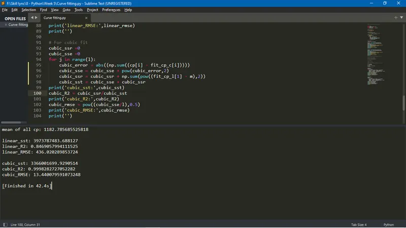
Result / Output :

Figure 1 -

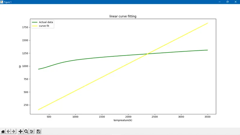
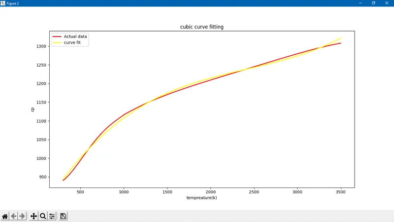
Figure 2 -

Question 5.

What needs to be done in order to make the curve fit perfect?

Answer :-

The degree of the equation of the curve is directly proportional the level of curve fit accuracy. As the number of coefficients increases the value estimated tend to follow the original curve.

Question 6.

Show empirically as to how well your curve has been fit.

Answer :-

AS per the above output, we can see that as the degree of the equation the linear curve fit plot looks a lot different to the original plot. In the quintic fit we can clearly see that the curves overlap signify well performed.