Week 5 - Curve fitting

Aim:

1. What does popt and pcov mean?
   
2. What does np.array(temperature) do?
3. What does the * in *popt mean?
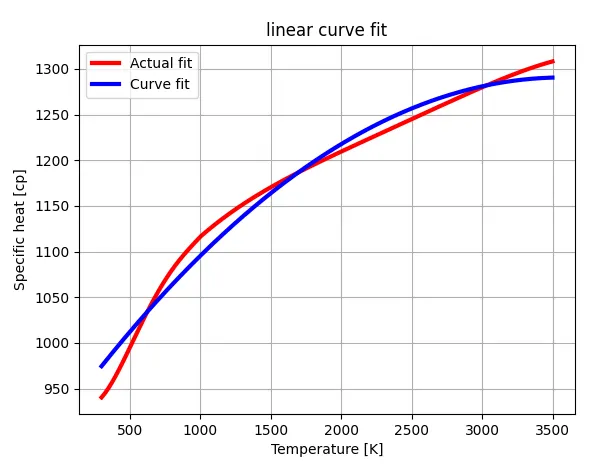
4. Write code to fit a linear and cubic polynomial for the Cp data. Explain if your results are good or bad.
5. What needs to be done in order to make the curve fit perfect?
6. Show empirically as to how well your curve has been fit?

THEORY:

Curve fitting is the process of constructing a curve or mathematical function, that has the best fit to a series of data points, possibly subject to constraints. Curve fitting can involve either interpolation, where an exact fit to the data is required, or smoothing, in which a smooth function is constructed that approximately fits the data. A related topic is regression analysis, which focuses more on questions of statistical interference such as how much uncertainty is present in a curve that is fit to data observed with random errors. Fitted curves can be used as an aid for data visualization, to infer values of a function where no data are available, and to summarize the relationships among two or more variables.

QUESTIONS:

1. What does popt and pcov mean? (Watch the video to get some context)

• popt is an array where all the coefficient of the equation is generated with respect to the polynomial degree.
• pcov is a 2D array that consists of the covariance of popt. Covariance gives the relation between two values, so here pcov gives the relation values between pop values.

2. What does np.array(temperature) do?

An array is a collection of items stored at contiguous memory locations. The idea is to store multiple items of the same type together. In python, the array command is stored in a module called numpy. in our challenge temperature is stored in form of an array with 3200 data.

3. What does the * in *popt mean?

• popt is an array which consists of all the coefficient of equation generated based on the degree of the polynomial
• *popt is the command which gives the same coefficient of the equation but it will multiply with e and give the output.

4. Write code to fit a linear and cubic polynomial for the Cp data. Explain if your results are good or bad.

Python Code to Fit a linear and cubic polynomial for Cp data.

LINEAR CURVE FIT:

import numpy as np
import matplotlib.pyplot as plt
from scipy.optimize import curve_fit

# Curve_fit(f,x,y)

file = open('data.txt', 'r')

def read_file():
    temperature = []
    cp = []

    for line in file:
        values = line.split(',')
        temperature.append(float(values[0]))
        cp.append(float(values[1]))

    return [temperature, cp]

def func(t, a, b, c):
    return a * pow(t, 2) + b * t + c

temperature, cp = read_file()
popt, pcov = curve_fit(func, temperature,
                       cp)  # popt i.e optimum parameters are returned which then can be passed to the funvction
fit_cp = func(np.array(temperature), *popt)

plt.plot(temperature, cp, linewidth=3, color='red')
plt.plot(temperature, fit_cp, linewidth=3, color='blue')
plt.xlabel('Temperature [K]')
plt.ylabel('Specific heat [cp]')
plt.legend(['Actual fit', 'Curve fit'])
plt.title('linear curve fit')
plt.grid()
plt.savefig('Linear fit')
plt.show()

OUTPUT PLOT:

CUBIC CURVE FIT:

import numpy as np
import matplotlib.pyplot as plt
from scipy.optimize import curve_fit

# Curve_fit(f,x,y)

file = open('data.txt', 'r')

def read_file():
    temperature = []
    cp = []

    for line in file:
        values = line.split(',')
        temperature.append(float(values[0]))
        cp.append(float(values[1]))

    return [temperature, cp]

def func(t, a, b, c, d):
    return a * pow(t, 3) + b * pow(t, 2) + c * t + d

temperature, cp = read_file()
popt, pcov = curve_fit(func, temperature,
                       cp)  # popt i.e optimum parameters are returned which then can be passed to the funvction
fit_cp = func(np.array(temperature), *popt)

plt.plot(temperature, cp, linewidth=3, color='red')
plt.plot(temperature, fit_cp, linewidth=3, color='blue')
plt.legend(['Actual_fit', 'Curve fit'])
plt.xlabel('Temperature [K]')
plt.ylabel('Specific heat [cp]')
plt.title('cubic curve fit')
plt.grid()
plt.savefig('cubic_fit')
plt.show()

OUTPUT PLOT:

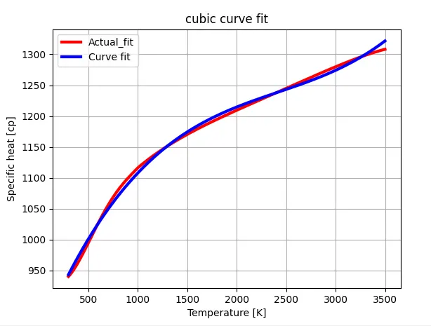
Curve with cubic equation has comparatively less percentage error than linear and quadratic equation as seen in the figure above. Thus, we conclude that with an increase in the order of the polynomial the error percentage decreases.

5. What needs to be done in order to make the curve fit perfectly?

The accuracy of the curve fit can be improved by increasing the degree of the polynomial. So, a 'Best fit' can be obtained by increasing the degree of the polynomial.

PERFECT FIT: The perfect fit is achieved when the geometric distances from the given points to the fitting curve are zero. This means that the curve fits perfectly on the points. To get a perfect fit we can increase to an order of the polynomials, this method increases the accuracy and reduces errors.

BEST FIT: The best fit is achieved when the geometric distances from the given points to the fitting curve are minimized, in the least-squares sense. Finding the best fit reduces the minimization of the objective function where denotes the fitting curve.

Upon finding a curve that satisfies the data points there are 4 quantities that help us measure the goodness of fit criteria or how well the equation is representing the data points.

The sum of squares due to error (SSE)

R-square

Adjusted R-square

Root mean squared error (RMSE)

SSE=∑(E2)

SSR=∑((Pcp−mean(cp))2

SST=SSE+SSR

R2=SSRS

RMSE=sqrt((SSE)/n)

Python Program to make curve fit perfect:

import numpy as np
import matplotlib.pyplot as plt
from scipy.optimize import curve_fit

# Curve_fit(f,x,y)

file = open('data.txt', 'r')

def read_file():
    temperature = []
    cp = []

    for line in file:
        values = line.split(',')
        temperature.append(float(values[0]))
        cp.append(float(values[1]))

    return [temperature, cp]

def func(t, a, b, c, d, e):
    return a * pow(t, 4) + b * pow(t, 3) + c * pow(t, 2) + d * t + e

temperature, cp = read_file()
popt, pcov = curve_fit(func, temperature,
                       cp)  # popt i.e optimum parameters are returned which then can be passed to the funvction
fit_cp = func(np.array(temperature), *popt)

plt.plot(temperature, cp, linewidth=3, color='red')
plt.plot(temperature, fit_cp, linewidth=3, color='blue')
plt.legend(['Actual fit', 'Curve fit'])
plt.xlabel('Temperature [K]')
plt.ylabel('Specific heat [cp]')
plt.title('perfect curve fit')
plt.grid()
plt.savefig('poly_fit')
plt.show()

OUTPUT PLOT:

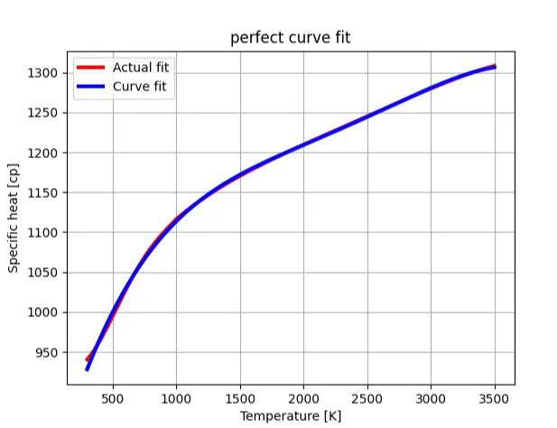
Therefore, In order to improve the curve fit, the degree of polynomial must be increased. Higher the degree of polynomial better is the curve fit obtained.