Week 2 Air standard Cycle

Aim:

To write the python code Based on the concepts of the forward kinematics routine, that can solve an otto cycle and make plots for it.

Objective:

1. Your code should create a PV diagram
2. You should output the thermal efficiency of the engine.

Problem statement:

Introduction of otto cycle:

An Otto cycle is an idealized thermodynamic cycle that describes the functioning of a typical spark ignition piston engine. It is the thermodynamic cycle most commonly found in automobile engines.

The Otto cycle is a description of what happens to a mass of gas as it is subjected to changes of pressure, temperature, volume, addition of heat, and removal of heat. The mass of gas that is subjected to those changes is called the system. The system, in this case, is defined to be the fluid (gas) within the cylinder. By describing the changes that take place within the system, it will also describe in inverse, the system's effect on the environment. In the case of the Otto cycle, the effect will be to produce enough network from the system so as to propel an automobile and its occupants in the environment.

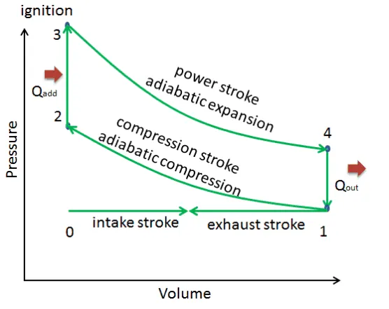
The processes are described by:

• Process 0–1 a mass of air is drawn into piston/cylinder arrangement at constant pressure.
• Process 1–2 is an adiabatic (isentropic) compression of the charge as the piston moves from bottom dead centre (BDC) to top dead centre (TDC).
• Process 2–3 is a constant-volume heat transfer to the working gas from an external source while the piston is at top dead centre. This process is intended to represent the ignition of the fuel-air mixture and the subsequent rapid burning.
• Process 3–4 is an adiabatic (isentropic) expansion (power stroke).
• Process 4–1 completes the cycle by a constant-volume process in which heat is rejected from the air while the piston is at bottom dead centre.
• Process 1–0 the mass of air is released to the atmosphere in a constant pressure process.

Engine kinematics:

During compression (1-2) and expansion (3-4) stroke, the change in volume is not linear. Rather given by engine kinematics whose relation is given by,

V/Vc=1+1/2(Cr-1) [R+1-cos θ (R^2-sin^2 θ) ^1/2]

Where,

V=volume trace at particular crank angle.

Vc=clearance volume of cylinder given by ratio of swept volume and compression ratio.

Vs=swept volume of cylinder as per the stroke length and bore diameter.

Cr=compression ratio.

R=constant given by ratio of length of connecting rod and crank pin radius.

a= half of stroke length.

θ = instantaneous crank angle.

Program code:

#Engine kinematics

import math
import matplotlib.pyplot as plt

def engine_kinematic(bore,stroke,con_rd,cr,start_crank,end_crank):
    #geomatric parameter
    a=stroke/2
    R=con_rd/a
    #volume parameters
    v_s=math.pi*(1/4)*pow(bore,2)*stroke
    v_c=v_s/(cr-1)

    sc=math.radians(start_crank)
    ec=math.radians(end_crank)
    num_values=50
    dtheta=(ec-sc)/(num_values-1)
    v=[]
    for i in range(0,num_values):
        theta=sc+i*dtheta
        term1=0.5*(cr-1)
        term2=R+1-math.cos(theta)
        term3=pow(R,2)-pow(math.sin(theta),2)
        term3=pow(term3,0.5)
        v.append((1+term1*(term2-term3))*v_c)
    return v
#inputs
p1=101325
t1=500
gamma=1.4
t3=2300
#geometric parameters
bore=0.1
stroke=0.1
con_rd=0.15
cr=8
#volume computation
v_s=(math.pi/4)*pow(bore,2)*stroke
v_c=v_s/(cr-1)
v1=v_c + v_s
# state point 2
v2=v_c
#p2v2^gamma=p1v1^gamma
p2=p1*pow(v1,gamma)/pow(v2,gamma)
#p2v2/t2=p1v1/t1 | rhs=p1v1/t1 | p2v2/t2=rhs | rhs=p2v2/rhs
rhs=p1*v1/t1
t2=p2*v2/rhs
v_compression= engine_kinematic (bore,stroke,con_rd,cr,180,0)
constant=p1*pow(v1,gamma)
p_compression=[]
for v in v_compression:
    p_compression.append(constant/pow(v,gamma))
#state point 3
v3=v2
#p3v3/t3=p2v2/t2 |rhs=p2v2/t2 |p3=rhs*t3/v3
rhs=p2*v2/t2
p3=rhs*t3/v3
v_expansion= engine_kinematic (bore,stroke,con_rd,cr,0,180)
constant=p3*pow(v3,gamma)
p_expansion=[]
for v in v_expansion:
    p_expansion.append(constant/pow(v,gamma))

#state point 4
v4=v1
#p4v4^gamma=p3v3^gamma
p4=p3*pow(v3,gamma)/pow(v4,gamma)
#p4v4/t4=rhs
t4=p4*v4/rhs

plt.plot([v2,v3],[p2,p3])
plt.plot(v_compression,p_compression)
plt.plot(v_expansion,p_expansion)
plt.plot([v4,v1],[p4,p1])
plt.xlabel('Volume')
plt.ylabel('Pressure')
plt.title('OTTO CYCLE')
plt.show()

#Thermal efficiency of ottocycle(te)
#input k=1.4
k=1.4
te=(1-1/pow(cr,(k-1)))*100
print (te)

Solution procedure:

• Before starting the program we used module like,importmath and import matplotlib.pyplot as plt.
• Then we used engine kinematics function return the volume (v)as arry of volumes which gradually changes during the isentropic process otherwise the isentropic curve would be linear which is not possible.
• Then initial condition are define as,

p1=101325 pa

t1=500

Gamma=1.4

t3=2300

• after that geometric parameter required for calculation are defined and volumes are computed.
• Then values of parameter at all states are computed.
• For Constant volume process
• Pv/t=constant
• for isentropic process
• (pv ^γ)=Constant
• Then this all formulae used for all compression and expansion process.
• Then using plot function the pressure vs volume graph is plotted.
• After that find thermal efficiency
• Thermal efficiency=[1-(1/cr^(gamma-1))]*100.

Output:-

PV plot is,

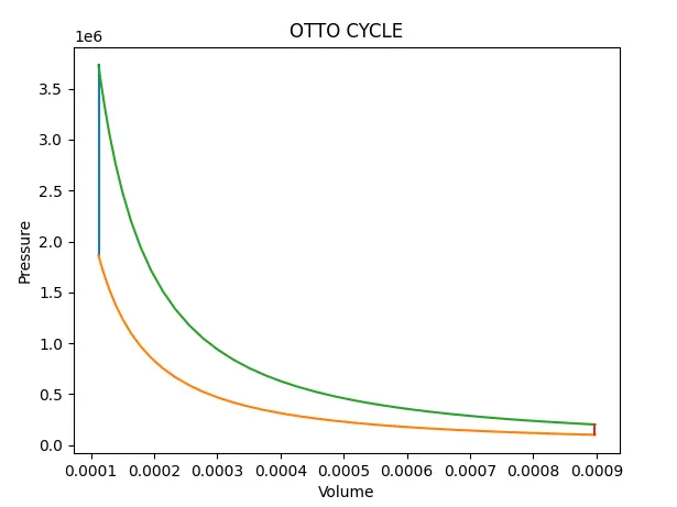
• Thermal efficiency is 56.47percent.in this result when compression ratio increases that time thermal efficiency also increased.

Result:

• The PV diagram was generated by using python.
• The thermal efficiency of the engine was calculated.