Week 5 - Curve fitting
Aim:
The aim is to give code for curve fitting for given data.
Procedure:
1. At first necessary modules such as math,matplotlib,numpy.scipy are imported to perform their respective functions.
2. Two functions are defined which return linear and cubic equations.
3. The following data is loaded into Python by placing it in right directory and a function read_file is created. For loop is used to run each line by using 'open' command with 'r' to read it.
4. From the data obtained, two individual column matrices of temperature and specific heat are derived.
5. For curve fitting, 'popt' and 'pcov are used as output for storing parameters obtained by 'curve fit' command which takes input as the required function(linear or cubic),temperature and Cp. Now, another variable namedfit_cp' stores the new values of Cp calculated by using temperature array.
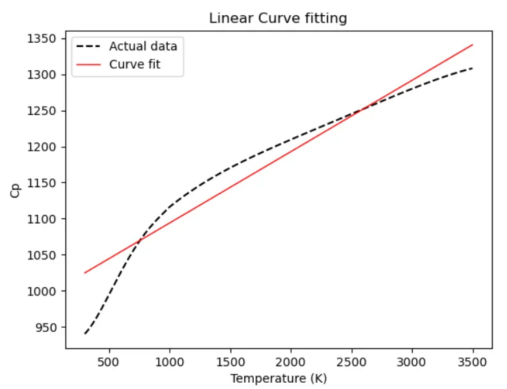
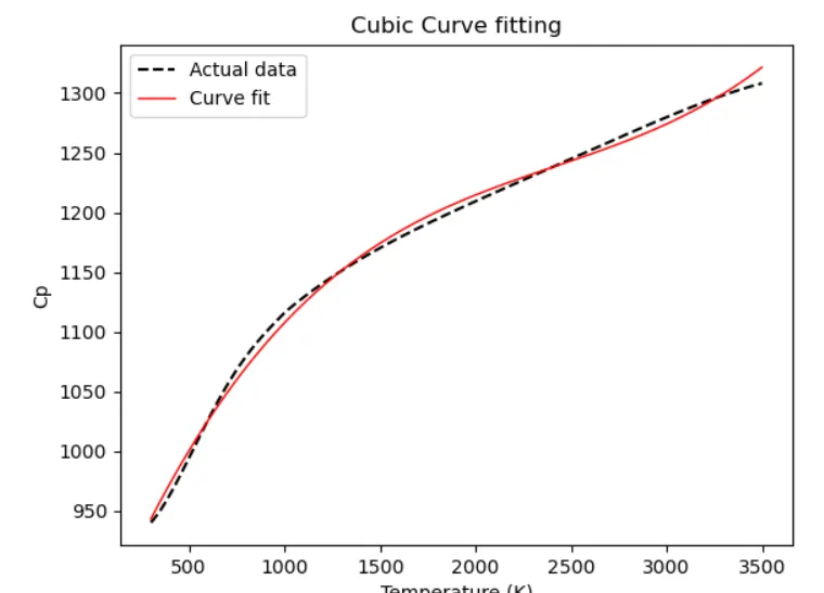
6. Plots of both raw dataset and predicted dataset are made and compared to find fitness characteristics for both the curves for both linear and cubic polynomial.
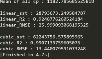
7. To measure the fitness characteristics for both the curves, various parameters such as SSE SSR,SST,R,RMSE are calculated. The plot which has highest n ^ 2 or closest to 1 is considered to be good fit.
# A program to measure fitness characteristics for the linear and cubic polynomial for the Cp data:

import math

import matplotlib.pyplot as plt

import numpy as np

from scipy.optimize import curve_fit

#Curve fit function

#Linear function

def function_0(t, a, b):

	return a * t + b

# Cubic function

def function_2(t, a, b, c, d) :

	return a * pow(t,3)+b * pow(t,2 ) + c*t +d

# Reading thermodynamic data file

def file() :

	temperature =[]

	cp=[]

	for line in open('data', 'r'):

		values= line.split(',')

		temperature.append(float(values[0]))

		cp.append(float(values[1]))

 return[temperature,cp]

#Main Program

temperature, cp = read_file()

popt, pcov = curve_fit(function_0, temperature, cp)

fit_cp_1 =function_0(np.array(temperature), *popt)

plt.figure(1)

plt.plot(temperature, cp, 'k--')

plt.plot(temperature, fit_cp_1,color='red', linewidth=1)

plt.legend(['Actual data', 'Curve fit'])

plt.xlabel('Temperature (K)')

plt.ylabel('cp')

plt.title('Linear Curve fitting')

plt.show()

popt, pcov = curve_fit(function_2, temperature, cp)

fit_cp_c = function_2(np.array(temperature), *popt)

plt.figure(3)

plt.plot(temperature, cp, 'k--')

plt.plot(temperature, fit_cp_c,color='red', linewidth = 1)

plt.legend(['Actual data', 'Curvefit'])

plt.xlabel('Temperature (K)')

plt.ylabel('Cp')

plt.title('Cubic Curve fitting')

plt.show()
'''

#Measuring the fitness characetristics of the curves

SSE (sum of error squared)

SSR (sum of squares of the regression)

SST=SSE+SSR

R^2=SSR/ST

RHSE=(SSE/l)^0.5

#Finding mean of Cp data

mean = (sum of all elements)/(total number of elements)'''

s = np.sum(cp)

l = np.size(cp)

m = s/1

print('Mean of all cp :',m)

print('')

# For Linear curve fit

linear_sse = 0

linear_ssr = 0

for i in range(1):

	linear_error=abs((np.sum((cp[i]-fit_cp_l[i]))))

	linear_sse = linear_sse=pow(linear_error,2)

	linear_ssr = linear_ssr+np.sum(pow((fit_cp_l[i]-m),2))

linear_sst = linear_sse + linear_ssr

print('linear_sst :',linear_sst)

linear_R2 = linear_ssr/linear_sst

print('linear_R2 :',linear_R2)

linear_rmse = pow((linear_sse/1),0.5)

print('linear_RMSE :',linear_rase)

print('')

# For Cubic curve fit

cubic_sse = 0

cubic_ssr = 0

for j in range(1):

	cubic_error=abs(np.sum((cp[i]-fit_cp_c[1])))

	cubic_sse = cubic_sse+(pow(cubic_error,2))

	cubic_ssr = cubic_ssr+np.sum(pow((fit_cp_c[i] - m),2))

cubic_sst = cubic_sse + cubic_ssr

print('cubic_sst :',cubic_sst)

cubic_R2 = cubic_ssr/cubic_sst

print('cubic_R2 :',cubic_R2)

cubic_rmse = pow((cubic_sse/1),0.5)

print('cubic RMSE :',cubic_rmse)
1. What does popt and pcov mean?
popt - array, pcov - 2d array
2. What does np.array(temperature) do?
it converts value of temp in data file to array
3. What does the * in *popt mean?
it denotes return coefficient stored in each popt array .
Result:
the code has been run and output are attached,