Python Challenge - Curve fitting
Curve Fitting
Objectives:
- Fit a linear and cubic polynomial for a given data and to get the best fit out of two fits.
- To get a perfect curve fit.
Solution:
Curve fitting is a process of constructing a curve, a mathematical model which possesses the closest proximity to the actual series of data with the slightest uncertainty.
There are various types of curve fitting processes:
- Linear Curve Fitting (Fitting of First-order polynomial to the data)
- Cubic Curve Fitting (Fitting of Third-order polynomial to the data)
- Higher Curve Fitting (Fitting of higher-order polynomial to the data)
- Split wise function(Use of same or different order polynomial to fit in the same path by breaking the path into subsets)
Parameters used to measure the fitness of the curve
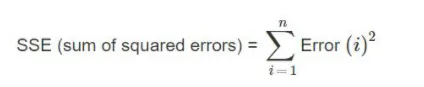
- SSE – The sum of squares due to error
- R-square
- Adjusted R-square
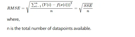
- Root mean square error (RMSE)
SSE is the sum of the squared differences between each observation and its group's mean. It can be used as a measure of variation within a cluster. If all cases within a cluster are identical the SSE would be equal to 0.
R-square This quantity that measures how successful the fit is in explaining the variation of the data. Put another way, R-square is the square of the correlation between the response values and the predicted response values. It is also called the square of the multiple correlation coefficient and the coefficient of multiple determination.

Where, SSR = Sum of squares of the regression
SST = SSR + SSE
Adjusted R-Square: This statistic uses the R-square statistic defined above, and adjusts it based on the residual degrees of freedom. The residual degrees of freedom are defined as the number of response values n minus the number of fitted coefficients m estimated from the response values. The adjusted R-square statistic can take on any value less than or equal to 1, with a value closer to 1 indicating a better fit.
Root Mean Squared Error: This statistic is also known as the fit standard error and the standard error of the regression An RMSE value closer to O indicates a better fit.
Problem Statement
. What do popt and pcov mean?
Ans: popt – It is a 2D array that contains the optimal values of the coefficients of a polynomial, in which the sum of squared residuals for a given data is minimized and it’s also used to extract the coefficients of a polynomial.
Pcov – It is also a 2D array that gives estimated values of covariance of coefficients of a polynomial. The diagonal elements of an array give the value of covariance of a coefficient with itself which is also known as the variance of that coefficient. Pcov can also be used to find the standard deviation of a given data set.
What does np.array(temperature) do?
Ans: This command is used to access the individual elements of the temperature array with the help of numpy module.
What does the * in *popt mean?
Ans: The * in *popt unpacks the popt array so that the values of the coefficient can be accessed.
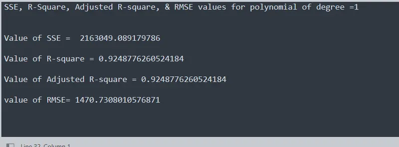
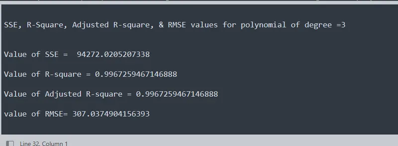
Write code to fit a linear and cubic polynomial for the Cp data. Explain if your results are good or bad.
import math
import matplotlib.pyplot as plt
import numpy as np
from scipy.optimize import curve_fit


# Reading thermodynamic data file
def read_file():
	temperature = []
	cp = []
	for line in open ('data','r'):
		values = line.split(',')
		temperature.append(float(values[0]))
		cp.append(float(values[1]))

	return [temperature,cp]


#Main function
temperature, cp = read_file()

#Performing Curve fit using linear polynomial

#Linear Curve fit function
def linear(T, a, b):
	return a*T + b

"""
Linear Equation = aT+b
"""

popt1, pcov1 = curve_fit(linear, temperature, cp)
linear_fit_cp = linear(np.array(temperature), *popt1)

#Comparing original data with the curve fit using linear polynomial

#Creating an empty figure
plt.figure(1)

#Creating a plot
plt.plot(temperature, cp, color='r', linewidth = 3, label = 'Original data')
plt.plot(temperature, linear_fit_cp, color = 'b', linewidth = 3, label = 'Curve Fit')

#Giving Title to plot
plt.title('Comparison of original data set and curve fit using linear ploynomial',color = 'k', fontsize = 10, fontweight = 'bold')

#Mentioning legend
plt.legend(['Actual data','Curve Fit'])

#Giving labels to the axis
plt.xlabel('Temperature[k]',fontsize = 10)
plt.ylabel('Specific Heat[kJ/kg-K]',fontsize = 10)

#Saving the plot as an image in PNG Format
plt.savefig('Curve fit using linear ploynomial.png')

#Making the plot visible
plt.show()


#Performing Curve fit using Cubic polynomial

#Cubic Curve fit function
def cubic(T, a, b, c, d):
	return a*pow(T,3) + b*pow(T,2) + c*T + d

"""
Linear Equation = aT^3+bT^2+cT+d
"""

popt2, pcov2 = curve_fit(cubic, temperature, cp)
cubic_fit_cp = cubic(np.array(temperature), *popt2)

#Comparing original data with the curve fit using cubic polynomial

#Creating an empty figure
plt.figure(2)

#Creating a plot
plt.plot(temperature, cp, color='r', linewidth = 3, label = 'Original data')
plt.plot(temperature, cubic_fit_cp, color = 'b', linewidth = 3, label = 'Curve Fit')

#Giving Title to plot
plt.title('Comparison of original data set and curve fit using cubic ploynomial',color = 'k', fontsize = 10, fontweight = 'bold')

#Mentioning legend
plt.legend(['Actual data','Curve Fit'])

#Giving labels to the axis
plt.xlabel('Temperature[k]',fontsize = 10)
plt.ylabel('Specific Heat[kJ/kg-K]',fontsize = 10)

#Saving the plot as an image in PNG Format
plt.savefig('Curve fit using cubic ploynomial.png')

#Making the plot visible
plt.show()

#Comparsion of fits for explantion of which results are better

#Program to calculate the fitness characteristics for curve fitting with linear and cubic polynomial

#No of datapoints
n = len(temperature)

#No of independent variables
k = 0

#Performing curve fitting using linear polynomial

#Calculation of fitness characteristics

#Goodness of curve
print('SSE, R-Square, Adjusted R-square, & RMSE values for polynomial of degree =1')
print('n')

#Sum of squares Errors(SSE)
SSE = np.sum(pow((np.array(np.array(cp) - np.array(linear_fit_cp))),2))
print('Value of SSE = ',SSE)
print('t')

#Sum of squares of regression(SSR)
SSR = np.sum(pow((np.array(np.array(linear_fit_cp) - np.mean(cp))),2))

#Total sum of squares(SST)
SST = SSE + SSR

#R-square
R_square = SSR/SST
print('Value of R-square =',R_square)
print('t')

#Adjusted R-square
Adjusted_R_square = 1 - ((1 - R_square) * (n-1)/(n-k-1))
print('Value of Adjusted R-square =',Adjusted_R_square)
print('t')

#Root Mean Square Error(RMSE)
RMSE = np.sqrt((np.sum(pow((np.array(np.array(cp)-np.array(linear_fit_cp))),2))))
print('value of RMSE=',RMSE)
print('n')
print('t')


#Performing curve fitting using cubic polynomial

#Calculation of fitness characteristics

#Goodness of curve
print('SSE, R-Square, Adjusted R-square, & RMSE values for polynomial of degree =3')
print('n')

#Sum of squares Errors(SSE)
SSE = np.sum(pow((np.array(np.array(cp) - np.array(cubic_fit_cp))),2))
print('Value of SSE = ',SSE)
print('t')

#Sum of squares of regression(SSR)
SSR = np.sum(pow((np.array(np.array(cubic_fit_cp) - np.mean(cp))),2))

#Total sum of squares(SST)
SST = SSE + SSR

#R-square
R_square = SSR/SST
print('Value of R-square =',R_square)
print('t')

#Adjusted R-square
Adjusted_R_square = 1 - ((1 - R_square) * (n-1)/(n-k-1))
print('Value of Adjusted R-square =',Adjusted_R_square)
print('t')

#Root Mean Square Error(RMSE)
RMSE = np.sqrt((np.sum(pow((np.array(np.array(cp)-np.array(cubic_fit_cp))),2))))
print('value of RMSE=',RMSE)
print('n')
print('t')
Explanation of the code:
- Importing the basic modules such as math, matplotlib, numpy and scipy.
- Defining the function ‘read_file’ which is used in reading the thermodynamic data file line by line by using for loop with the line as a counter variable and storing data i.e temperature and specific heat into two arrays temperature and cp respectively after splitting each line on the basis of comma ‘line.split(‘,’)’.
- The function read_file is then called to get the array's temperature and cp.
- Function linear is used to define the linear polynomial which is going to be fitted in the data.
- ‘popt’ and ‘pcov’ are obtained as output arguments by calling the inbuilt function ‘curve_fit’ and passing the function linear and the arrays(temperature and cp) inside curve_fit as inputs.
- Then the new value of cp is calculated according to the linear polynomial (linear_fit_cp) by calling the function ‘linear’, and passing the temperature array element-wise using numpy module and all the coefficients of the linear polynomial using *popt as the input argument.
- A figure of comparison is obtained then between the original dataset plot and the curve fit plot in a single figure window.
- Similarly, the cubic polynomial is fitted to the data except in the fourth step in which a cubic polynomial is defined which is further passed as an input argument inside the curve_fit function and used for calculating the new value of cp i.e ‘cubic_fit_cp’. Then a figure of comparison is obtained.
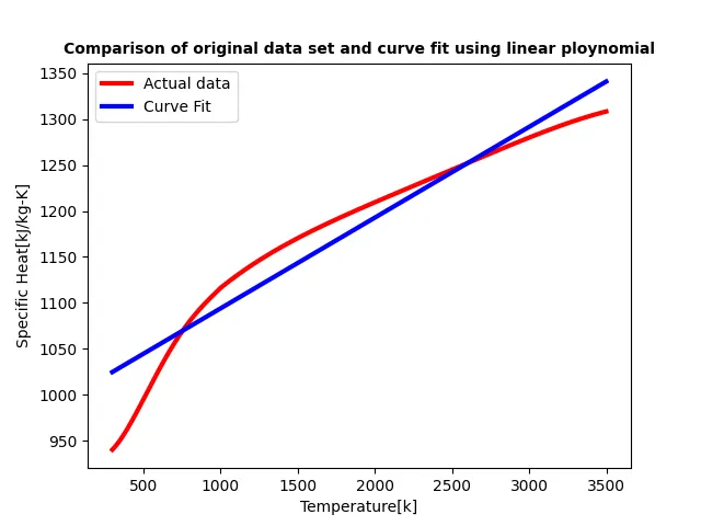
The plot of comparison of original data set and curve fit data using linear polynomial:
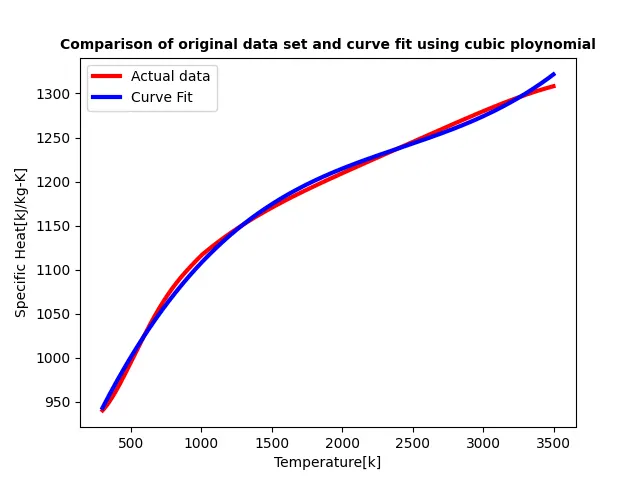
The plot of comparison of original data set and curve fit data using cubic polynomial:
What needs to be done in order to make the curve fit perfect?
Ans: The order of the polynomial can be increased to make the curve fit perfectly. We may also use split wise method to get a perfectly more fit curve. The advantage of using this method over higher-order polynomial is that a perfect fit can be obtained using the lower-order polynomial.
Code for split wise method:
import math
import matplotlib.pyplot as plt
import numpy as np
from scipy.optimize import curve_fit

# Reading thermodynamic data file
def read_file():
	temperature = []
	cp = []
	for line in open ('data','r'):
		values = line.split(',')
		temperature.append(float(values[0]))
		cp.append(float(values[1]))

	return [temperature,cp]


#Main function
temperature, cp = read_file()

#Preparing Temperature and cp arrays in 8 different ranges
temperature1 = temperature[0:400]
cp1 = cp[0:400]

temperature2 = temperature[401:800]
cp2 = cp[401:800]

temperature3 = temperature[801:1200]
cp3 = cp[801:1200]

temperature4 = temperature[1201:1600]
cp4 = cp[1201:1600]

temperature5 = temperature[1601:2000]
cp5 = cp[1601:2000]

temperature6 = temperature[2001:2400]
cp6 = cp[2001:2400]

temperature7 = temperature[2401:2800]
cp7 = cp[2401:2800]

temperature8 = temperature[2801:3200]
cp8 = cp[2801:3200]

#Now performing curve fit using cubic polynomial

#Cubic Curve fit function
def qua(T, a, b, c):
	return (a*pow(T,2) + b*T + c)

"""
Linear Equation = aT^2+bT+c
"""

#Curve fitting for all ranges

popt1, pcov1 = curve_fit(qua, temperature1, cp1)
split_wise_fit_cp1 = qua(np.array(temperature1), *popt1)

popt2, pcov2 = curve_fit(qua, temperature2, cp2)
split_wise_fit_cp2 = qua(np.array(temperature2), *popt2)

popt3, pcov3 = curve_fit(qua, temperature3, cp3)
split_wise_fit_cp3 = qua(np.array(temperature3), *popt3)

popt4, pcov4 = curve_fit(qua, temperature4, cp4)
split_wise_fit_cp4 = qua(np.array(temperature3), *popt4)

popt5, pcov5 = curve_fit(qua, temperature5, cp5)
split_wise_fit_cp5 = qua(np.array(temperature3), *popt5)

popt6, pcov6 = curve_fit(qua, temperature6, cp6)
split_wise_fit_cp6 = qua(np.array(temperature6), *popt6)

popt7, pcov7 = curve_fit(qua, temperature7, cp7)
split_wise_fit_cp7 = qua(np.array(temperature7), *popt7)

popt8, pcov8 = curve_fit(qua, temperature8, cp8)
split_wise_fit_cp8 = qua(np.array(temperature8), *popt8)

#Creation of split_wise_fit_cp array
split_wise_fit_cp = np.concatenate((split_wise_fit_cp8, split_wise_fit_cp7, split_wise_fit_cp6, split_wise_fit_cp5, split_wise_fit_cp4, split_wise_fit_cp3, split_wise_fit_cp2, split_wise_fit_cp1))

#Comparing original data with the curve fit using cubic polynomial

#Creating an empty figure
plt.figure()

#Creating a plot

plt.plot(temperature, cp, color = 'b', linewidth = 3, label = 'original data')


plt.plot(temperature1,cp1, color = 'r', linewidth = 3, label = 'curve fit')
plt.plot(temperature2,cp2, color = 'r', linewidth = 3)
plt.plot(temperature3,cp3, color = 'r', linewidth = 3)
plt.plot(temperature4,cp4, color = 'r', linewidth = 3)
plt.plot(temperature5,cp5, color = 'r', linewidth = 3)
plt.plot(temperature6,cp6, color = 'r', linewidth = 3)
plt.plot(temperature7,cp7, color = 'r', linewidth = 3)
plt.plot(temperature8,cp8, color = 'r', linewidth = 3)

#plt.plot(temperature, split_wise_fit_cp)

#Giving Title to plot
plt.title('Comparison of original data set and curve fit using cubic ploynomial with split wise method',color = 'k', fontsize = 10, fontweight = 'bold')

#Mentioning legend
plt.legend(['Actual data','Curve Fit'])

#Giving labels to the axis
plt.xlabel('Temperature[k]',fontsize = 10)
plt.ylabel('Specific Heat[kJ/kg-K]',fontsize = 10)

#Saving the plot as an image in PNG Format
plt.savefig('Curve fit using split wise method cubic ploynomial.png')

#Making the plot visible
plt.show() 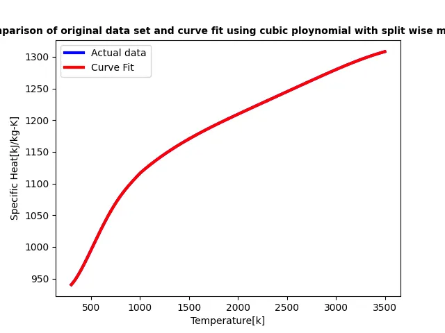
Errors faced while
- Initially, I didn’t get what the question demands.
- Some typo errors.
- The problem in understanding the concept of Fitness of the curve