Genetic Algorithm

Aim:

To understand the concept of genetic algorithm and calculate the global maxima using the stalagmite function.

Questions to be answered

• Write a code in MATLAB to optimize the stalagmite function and find the global maxima of the function.
• Clearly explain the concept of genetic algorithm in your own words and also explain the syntax for ga in MATLAB in your report.
• Make sure that your code gives the same output, even if it is made to run several times.
• Plot graphs for all 3 studies and for F maximum vs no. of iterations. Title and axes labels are a must, legends could be shown if necessary.

A genetic algorithm is a method of solving both constrained and unconstrained optimization problems by randomly selecting any individuals from the current data/population and using them as a parent to produce/calculate data for the next generation. So, basically, it’s an optimization technique.

The algorithm repeatedly modifies a population of individual solutions.

We can use the genetic algorithm method to solve problems that are not well suited for standard optimization algorithms including problems in which the objective function is discontinuous, non-differentiable, stochastic or highly nonlinear.

GA is different from classical, derived-based, optimization algorithms in two ways:

1. The classical Algorithm generates a single point at each iteration while GA generates a population of points at iteration.
2. IN CA the sequence of points approaches to an optimal solution while in GA the best point in the population approaches an optimal solution.
3. CA selects the next point in the sequence by a deterministic computation while in GA the next population is selected by computation which uses random number generators.

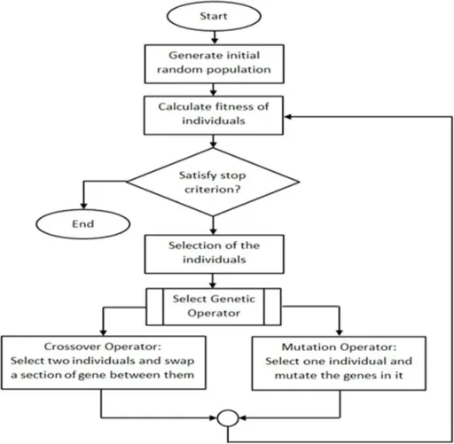
The following steps are to be followed to create a GA:

1. The algorithm begins by creating a random initial population.
2. The algorithm then creates a sequence of new populations. At each step, the algorithm uses the individuals in the current generation to create the next population. To create the new population, the algorithm performs the following steps:
   1. Scores each member of the current population by computing its fitness value. These values are called the raw fitness scores.
   2. Scales the raw fitness scores to convert them into a more usable range of values. These scaled values are called expectation values.
   3. Selects members, called parents, based on their expectations.
   4. Some of the individuals in the current population that have lower fitness are chosen as elite. These elite individuals are passed to the next population.
   5. Produces children from the parents. Children are produced either by making random changes to a single parent—mutation—or by combining the vector entries of a pair of parents—crossover.
   6. Replaces the current population with the children to form the next generation.
3. The algorithm stops when one of the stopping criteria is met.
4. The algorithm takes modified steps for linear and integer constraints.
5. The algorithm is further modified for nonlinear constraints.

Syntax of ga:

The ga syntax in Matlab is used to find the minimum of a function using a genetic algorithm. There are several ways to define the ga function depending on the problem being solved.

x= ga(fun.nvars)

where, X = optimal solution/variables; fun =Objective function; nvars =Number of variables; Sometimes [x,fvall] is used instead of X where 'fval' gives objective function value at the solution

x=ga(fun. nvars, A, B, Aeq, Beq, lb, ub)

where, A, B Linear inequality constraints; Aeq, Beq= Linear equality constraints If there are no linear equalities and inequalities, then A, B, Aeq, Beq are set to '[]'.

x=ga(fun .nvars. A. B, Aeq, Beq, lb, ub. nonlcon. IntCon ,options)

where, nonlcon =Nonlinear constraints; IntCon= Integer Values; options= Optimization options. If there are no nonlinear constraints and integer values, the nonlcon and IntCon are set to ‘[]’.

Stalagmite function:

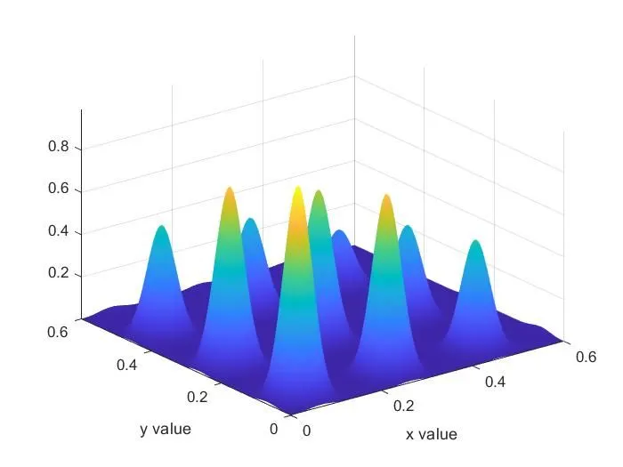
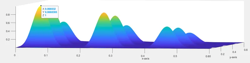
It is a function with which we find out the values of local, global maxima, and minima of a given particular function. It generates the 3D model in the form of Stalagmite rocks that’s why it is named as stalagmite function.

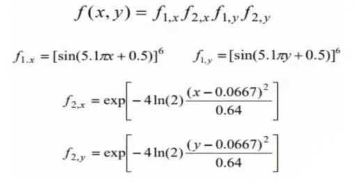
The mathematical equation is given as:

MATLAB PROGRAM:

Stalagmite function:
%Defining Stalagmite function
function [f] = stalagmite(input_vector)
x = input_vector(1);
y = input_vector(2);

t1 = (sin((5.1*pi*x)+0.5))^6;
t2 = (sin((5.1*pi*y)+0.5))^6;
t3 = exp(-4*log(2)*((x-0.0667)^2)/0.64);
t4 = exp(-4*log(2)*((y-0.0667)^2)/0.64);

f = -(t1*t2*t3*t4);  %Negative sign inverts the objective function
end

Genetic Algorithm Code:
clear all
close all
clc

%Defining our search space
x = linspace(0,0.6,150);
y = linspace(0,0.6,150);

%Number of cases
n=50;

%Creating a 2-d mesh
[xx yy] = meshgrid(x,y);

%Evaluating the salagmite function
for i=1:length(xx)
    for j=1:length(yy)
        input_vector(1)=xx(i,j);
        input_vector(2)=yy(i,j);
        f(i,j)=stalagmite(input_vector);
    end
end

%Study1 Statistical Behaviour

tic
for i=1:n
    [inputs,fopt(i)] = ga(@stalagmite,2);
    xopt(i) = inputs(1);
    yopt(i) = inputs(2);
end

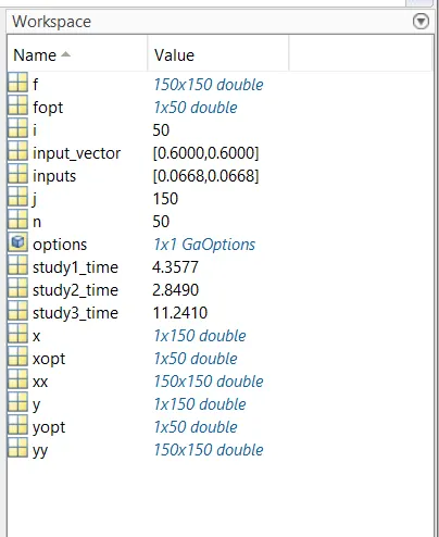
study1_time = toc

figure(1)
subplot(2,1,1)
hold on
surfc(xx,yy,-f)
shading interp
xlabel('x-axis')
ylabel('y-axis')
title('Unbound inputs')
plot3(xopt,yopt,-fopt,'marker','o','markersize',5,'MarkerFaceColor','r')
subplot(2,1,2)
plot(-fopt)
xlabel('No of Iterations')
ylabel('Function maximum')

%Study2 Statistical Behaviour with upper and lower bounds

tic
for i=1:n
    [inputs,fopt(i)] = ga(@stalagmite,2,[],[],[],[],[0;0],[1;1]);
    xopt(i) = inputs(1);
    yopt(i) = inputs(2);
end

study2_time = toc

figure(2)
subplot(2,1,1)
hold on
surfc(xx,yy,-f)
shading interp
xlabel('x-axis')
ylabel('y-axis')
title('Upper and lower bounds')
plot3(xopt,yopt,-fopt,'marker','o','markersize',5,'MarkerFaceColor','r')
subplot(2,1,2)
plot(-fopt)
xlabel('No of Iterations')
ylabel('Function maximum')

%Study3 Statistical Behaviour with increasing iterations of ga

options = optimoptions('ga');
options = optimoptions(options,'PopulationSize',300);

tic
for i=1:n
    [inputs,fopt(i)] = ga(@stalagmite,2,[],[],[],[],[0;0],[1;1],[],[],options);
    xopt(i) = inputs(1);
    yopt(i) = inputs(2);
end
study3_time = toc

figure(3)
subplot(2,1,1)
hold on
surfc(xx,yy,-f)
shading interp
xlabel('x-axis')
ylabel('y-axis')
title('Statistical behaviour with increasing iterations')
plot3(xopt,yopt,-fopt,'marker','o','markersize',5,'MarkerFaceColor','r')
subplot(2,1,2)
plot(-fopt)
xlabel('No of Iterations')
ylabel('Function maximum')

Code explanation:

1. We started the code with clear all, close all, clc and then we made the arrays ‘x’ , ‘y’ and divided the values into 150 equal parts by using ‘linspace’ command.
2. The number of cases/iterations has been defined to 50.
3. A 2D mesh of x and y is created using ‘meshgrid’ command.
4. For Evaluting statalgmite function a ‘for loop’ is created in which for each value of ‘i’ another ‘for loop’ is created to initialise the value of ‘j’.
5. Then, the input vector valued ‘xx’ and ‘yy’ is defined to use these input values in stalagmite function.
6. Now we need to obtain the result for 3 different cases first with no restrictions, second with upper and lower bounds, third with increasing the number of iterations.
7. For this we will use ‘for loop’ in which ga syntax will give the values for inputs and optimum maximum value.
8. The stalagmite function is called in the ga syntax and the number of variables ‘nvars’ are 2.
9. T o know how much time is taken to complete the 50 iterations ‘tic’ and ‘toe’ command is used before and after the loop.
10. Now the function is plotted by using the ‘surfc’ command foe ‘xx’, ‘yy’, and ‘function o/p’.
11. ‘Shading interp’ is used to obtain a smooth plot.
12. The subplot(2,1,1) is used to plot multiple plot on same figure which also divides the figure in grid of 2x1 and axes to be placed at 1.
13. The ‘plot3’ command is used to plots the 3D points at ‘xopt’, ‘yopt’, and ‘function optimum value’ with red colour and circular dot. Now in the same figure the values of optimum function(fopt) are plotted for 50 iterations.
14. But the results of the first case is different every time we run the program. To get the same value each time we need to restrict the program with upper and lower bound.
15. The code will be almost same the only difference will be in the syntax of ga as in the algorithm we have provided the limits with upper limit [1:1] and lower limit[0:0].
16. After running the program it is observed that the results is still not the same every time we run the program. So, to solve this problem we will increase the number of iteration to 300 and for this case, the syntax “options=optimoptions(‘slovername’,’name’,’value’) is used which retures with named parameters ‘Populations’ with altered values ‘300’. The syntax of ga will contain the ‘options’ term and rest of the code is same as study2.

Results:

Study1 – Statistical Behaviour with unbound inputs:

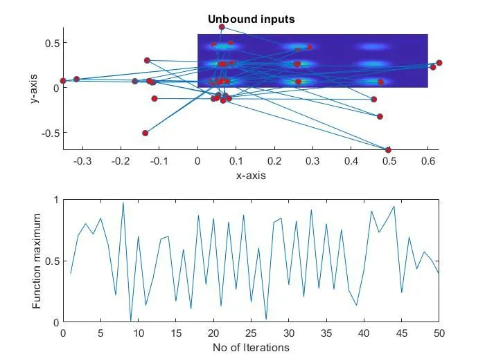
In the plot, we can observe how the random sampling of the genetic algorithm generates a new optimum value for the function every time it runs.

Study2 – Statistical Behaviour with upper and lower bounds:

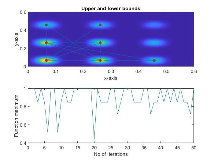
In this case, we can observe the convergence of x & y. The number of red dots are also less compared to study1.

Study3 – Statistical Behaviour with increasing no of iterations in GA

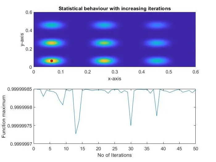
In this case, the no of iterations has been increased to 300 to find the global maxima of the function. Only one red dot appears and that’s the global maxima.

Reference links:

https://in.mathworks.com/help/gads/how-the-genetic-algorithm-works.html

https://in.mathworks.com/discovery/genetic-algorithm.html

https://in.mathworks.com/help/gads/ga.html

https://skill-lync.com/knowledgebase/genetic-algorithm-explained