Week 5 - Curve fitting
1) What do popt and pcov mean?
The popt and pcov are generally known as the output values of the python’s ‘curve fit’ inbuilt function.
popt- The return value popt contains the best-fit values of the parameters or coefficient of a polynomial so that the sum of the squared residuals of f(xdata, *popt) – ydata is minimized.
pcov- It is a second return argument and a 2D array that estimates covariance of popt. The diagonals provide the variance of the parameter estimate. The return value pcov contains the covariance (error) matrix for the fit parameters.
2) What does np.array(temperature) do?
This function stores the values of temperature in the form of an array. The command np.array (temperature) helps to access the elements present in the temperature array or temperature list with the help of numpy module.
3) What does the * in *popt mean?
The function stores the values of the constant coefficients or the best parameters of the polynomial (e.g., a, b, c) in the 2D array popt.
4) Write code to fit a linear and cubic polynomial for the Cp data. Explain if your results are good or bad.
Curve fitting is the process of constructing a curve or mathematical function, that has the best fit to a series of data points possibly subject to constraints. Curve fitting can involve either interpolation, where an exact fit to the data is required, or smoothing, in which a "smooth" function is constructed that approximately fits the data. A related topic is regression analysis which focuses more on questions of statistical inference such as how much uncertainty is present in a curve that is fit to data observed with random errors. Fitted curves can be used as an aid for data visualization to infer values of a function where no data are available and to summarize the relationships among two or more variables. Extrapolation refers to the use of a fitted curve beyond the range of the observed data and is subject to a degree of uncertainty since it may reflect the method used to construct the curve as much as it reflects the observed data.
Fitting functions to data points:
The first-degree polynomial equation
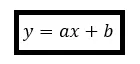
is a line with slope ‘a’. A line will connect any two points, so a first-degree polynomial equation is an exact fit through any two points with distinct x coordinates.
If the order of the equation is increased to a second-degree polynomial, the following results:
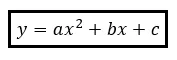
This will exactly fit a simple curve to three points.
If the order of the equation is increased to a third-degree polynomial, the following is obtained:-
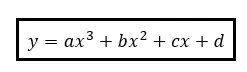
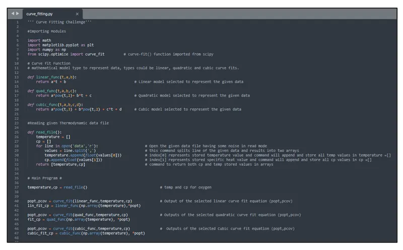
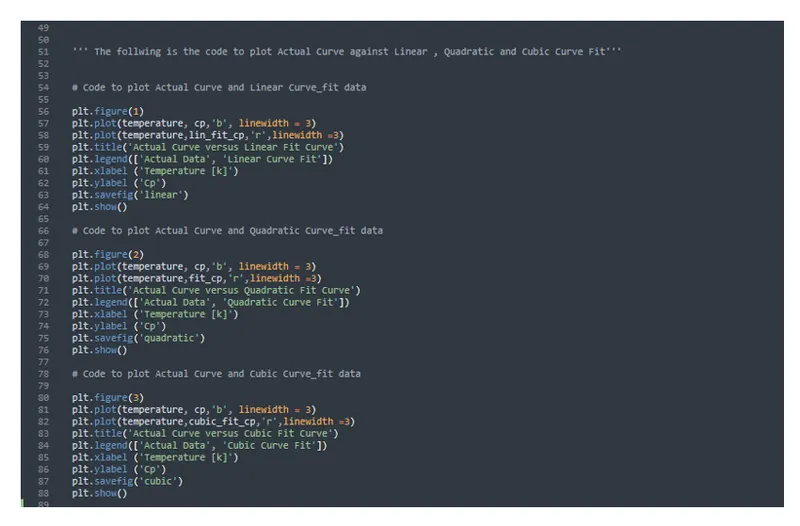
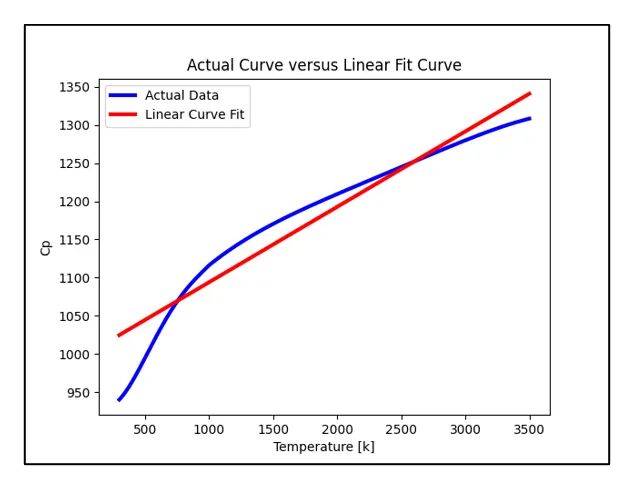
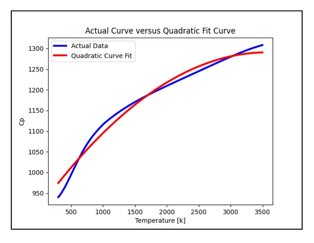
The python program to fit a linear and cubic polynomial for the Cp data is attached in the following figures.
5) What needs to be done in order to make the curve fit perfect?
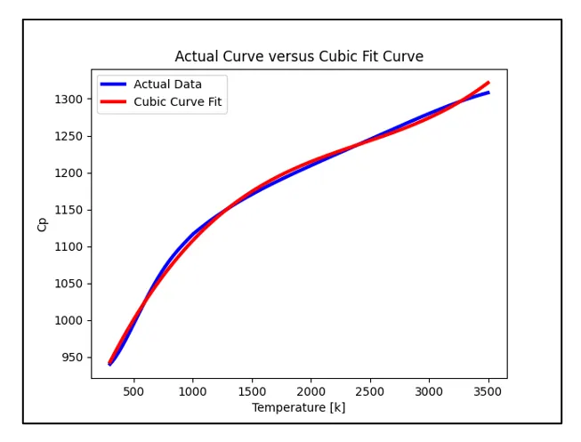
The best curve fit graphs were plotted using linear, quadratic, and cubic polynomial equations as per the challenge requirements. From the plotted graphs, it can be seen that the Linear curve and Quadratic fit curves deviate quite a much from the actual curve. However, the cubic fit curve slightly matches the actual curve meaning with an increment in the order of the polynomial equation the curve fits closely with the actual curve. In order to make the curve fit perfect, we have to keep increasing the order of the polynomial equation until it exactly matches and follows the pattern of the given actual cp (specific heat) versus temperature curve.
Another method could be the usage of split-wise polynomial equations.
6) Show empirically as to how well your curve has been fit.
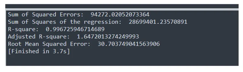
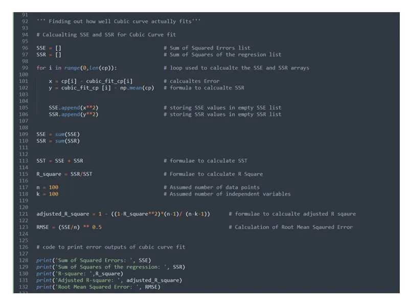
Since the linear and Quadratic fit curves do not follow the pattern of the actual curve and only the cubic fit curve has shown some resemblance, the following is the python program written to check how well the cubic curve really fits.
The SSE(sum of squared errors), SSR (sum of squares of the regression), SST, R Square, Adjusted R Square, and RMSE (root mean squared error) values were calculated. The Value of the R Square was found to be 0.997 (>0.95) indicating that the cubic fit curve is a good fit and acceptable.
Appendix:
''' Curve Fitting Challenge'''

#Importing Modules

import math
import matplotlib.pyplot as plt
import numpy as np
from scipy.optimize import curve_fit         # curve-fit() function imported from scipy

# Curve fit Function
# mathematical model type to represent data, types could be linear, quadratic and cubic curve fits.

def linear_func(t,a,b):
	return a*t + b                                # Linear model selected to represent the given data

def quad_func(t,a,b,c):
	return a*pow(t,2)+ b*t + c                    # Quadratic model selected to represent the given data

def cubic_func(t,a,b,c,d):
	return a*pow(t,3) + b*pow(t,2) + c*t + d      # Cubic model selected to represent the given data


#Reading given Thermodynamic data file

def read_file():
	temperature = []
	cp = []
	for line in open('data','r'):                      # Open the given data file having some noise in read mode
		values = line.split(',')                       # this command splits line of the given data and results into two arrays
		temperature.append(float(values[0]))           # index[0] represents stored temperature value and command will append and store all temp values in temperature =[]
		cp.append(float(values[1]))                    # index[1] represents stored specific heat value and command will append and store all cp values in cp =[]
	return [temperature,cp]                            # command to return both cp and temp stored values in arrays


# Main Program #

temperature,cp = read_file()                                  # temp and cp for oxygen


popt,pcov = curve_fit(linear_func,temperature,cp)             # Output of the selected linear curve fit equation (popt,pcov)
lin_fit_cp = linear_func(np.array(temperature),*popt)

popt,pcov = curve_fit(quad_func,temperature,cp)               # Outputs of the selected quadratic curve fit equation (popt,pcov)
fit_cp = quad_func(np.array(temperature), *popt)

popt,pcov = curve_fit(cubic_func,temperature,cp)              #  Outputs of the selected Cubic curve fit equation (popt,pcov)
cubic_fit_cp = cubic_func(np.array(temperature), *popt)


''' The follwing is the code to plot Actual Curve against Linear , Quadratic and Cubic Curve Fit'''


# Code to plot Actual Curve and Linear Curve_fit data

plt.figure(1)
plt.plot(temperature, cp,'b', linewidth = 3)
plt.plot(temperature,lin_fit_cp,'r',linewidth =3)
plt.title('Actual Curve versus Linear Fit Curve')
plt.legend(['Actual Data', 'Linear Curve Fit'])
plt.xlabel ('Temperature [k]')
plt.ylabel ('Cp')
plt.savefig('linear')
plt.show()

# Code to plot Actual Curve and Quadratic Curve_fit data

plt.figure(2)
plt.plot(temperature, cp,'b', linewidth = 3)
plt.plot(temperature,fit_cp,'r',linewidth =3)
plt.title('Actual Curve versus Quadratic Fit Curve')
plt.legend(['Actual Data', 'Quadratic Curve Fit'])
plt.xlabel ('Temperature [k]')
plt.ylabel ('Cp')
plt.savefig('quadratic')
plt.show()

# Code to plot Actual Curve and Cubic Curve_fit data

plt.figure(3)
plt.plot(temperature, cp,'b', linewidth = 3)
plt.plot(temperature,cubic_fit_cp,'r',linewidth =3)
plt.title('Actual Curve versus Cubic Fit Curve')
plt.legend(['Actual Data', 'Cubic Curve Fit'])
plt.xlabel ('Temperature [k]')
plt.ylabel ('Cp')
plt.savefig('cubic')
plt.show()


''' Finding out how well Cubic curve actually fits'''

# Calcualting SSE and SSR for Cubic Curve fit

SSE = []                                 # Sum of Squared Errors list
SSR = []                                 # Sum of Squares of the regression list

for i in range(0,len(cp)):               # loop used to calcualte the SSE and SSR arrays

	x = cp[i] - cubic_fit_cp[i]          # calcualtes Error
	y = cubic_fit_cp [i] - np.mean(cp)   # formula to calcualte SSR


	SSE.append(x**2)                     # storing SSE values in empty SSE list
	SSR.append(y**2)                     # storing SSR values in empty SSR list


SSE = sum(SSE)
SSR = sum(SSR)


SST = SSE + SSR                          # formulae to calculate SST

R_square = SSR/SST                       # Formulae to calculate R Square

n = 100                                  # Assumed number of data points
k = 100                                  # Assumed number of independent variables


adjusted_R_square = 1 - ((1-R_square**2)*(n-1)/ (n-k-1))      # formulae to calcualte adjusted R sqaure

RMSE = (SSE/n) ** 0.5                                         # Calculation of Root Mean Sqaured Error


# code to print error outputs of cubic curve fit

print('Sum of Squared Errors: ', SSE)
print('Sum of Squares of the regression: ', SSR)
print('R-square: ',R_square)
print('Adjusted R-square: ', adjusted_R_square)
print('Root Mean Squared Error: ', RMSE)