Week 5 - Curve fitting

AIM:
To fit the mathematical curve for the given thermodynamic data and to understand the steps for
getting better curve fits for the data provided under the stated constraints.

THEORY:
Curve fitting is one of the main concerns in recent studies to get the relational behavior between
the two data sets and their dependence on one another .The curve is best when the sum of the
squares between the actual and predicted data is least . The procedure is first expressing the
required form including variables and constant in a function then from scipy.optimize library we
use curve fit function to get the numeric values for the constant in the stated expression. Then
pass this, get the values and then find the suitable curve with the expression by increasing the
polynomial order and we can also introduce transcendental equations for better interpretations.

OBJECTIVE:
The main motive of the program is to fit the curve for the given data which has the least sum of
squares and to know the deciding factors for the curve fit.

BODY OF THE CONTENT :
Task 1-popt is an array of the optimal numerical constants stated in the expression for fitting
the curve for the data. This is found under the least square concept. while pcov is an array of
estimated covariance in the parameters of popt.
Task 2 -np.array(temperature) is a function in which the list type temperature is converted into
ndarray type / it stores the temperature in array format.
Task 3- *in *popt is used to return multiple parameters in single statement the * notation makes
this possible by returning more than one parameters like in popt array with the single statement.
Task 4 - Python is used as programming language

"""
program to plot the interpolated curve for the given data and their dependence 
written by GAGAN.k
mail id- [email protected]
 in this program we are going to interpolate and fit a curve for the given  raw data first with linear curve fit 
 and then with cubic polynomial curve by increasing the polynomial order we can get the best fit for the data without 
 even different curves under different interval , curve fit functionality is used from the scipy.optimize folder .
 
"""

#importing suitable libraries for the functionalities 
import numpy as np 
import math 
import matplotlib.pyplot as plt 
from  scipy.optimize import curve_fit

# linear curve fit for the data 
def fun_1(i,z,k):
	return z*i+k
#cubic curve fit for the data 
def fun_3(i_3,a_3,b_3,c_3,d_3):
	return (i_3**3)*a_3+(i_3**2)*b_3+(i_3)*c_3+d_3

#higher order curve filt for the data
def fun_6(x,m,c,d,e,h,g,j):
	return (d*pow(x,2))+m*x+c+(e*x**3)+(h*x**4)+(g*x**5)+(j*x**6)

#getting the thermodynamic data from the file and storing it in the suitable list
d_=open("data","r")
temp=[]   #temperature list
cp=[]     #specific heat value at constant pressure

for line in d_:
	a,b=line.split(',')
	temp.append(float(a)) #appending the values at each line 
	cp.append(float(b))   #appending the values at each line 


#----------------------------------------

#linear curve fit and plotting them over the graph
s,t=curve_fit(fun_1,np.array(temp),np.array(cp))
f_1=fun_1(np.array(temp),*s)
plt.savefig("linear")
plt.xlabel("temperature")
plt.ylabel("cp")
plt.title("linear curve fit")
plt.plot(temp,cp)
plt.plot(temp,f_1,"r--")
plt.legend(["actual data"," fitted "])
plt.show()
r_1=f_1 -cp              #difference between predicted cp and actual cp value
m1=np.array(r_1)
m1=m1*m1                #squaring the difference values
m1=np.mean(m1)
print(m1," mean of the squared residuals in linear curve fit  r_1 ")

#------------------------------------
#cubic curve fit  and plotting them over the graph
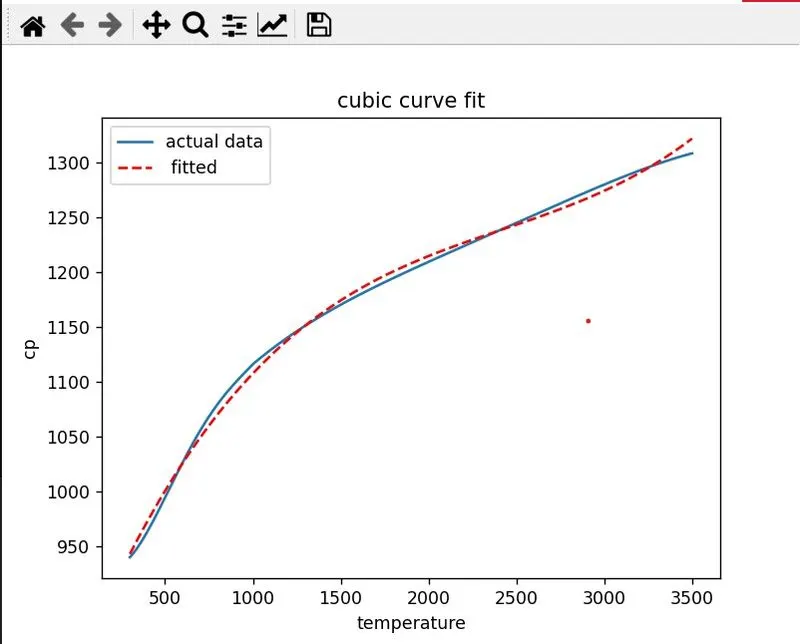
s_3,t_3=curve_fit(fun_3,np.array(temp),np.array(cp))
f_3=fun_3(np.array(temp),*s_3)
plt.savefig("cubic")
plt.xlabel("temperature")
plt.ylabel("cp")
plt.title("cubic curve fit")
plt.plot(temp,cp)
plt.plot(temp,f_3,"r--")
plt.legend(["actual data"," fitted "])
plt.show()
r_3=f_3 -cp             #difference between predicted cp and actual cp value
m3=np.array(r_3)
m3=m3*m3                #squaring the difference values
m3=np.mean(m3)
print(m3," mean of the squared residuals in cubic curve fit r_3")
#-----------------------------------

# higher polynomial curve fit  and plotting them over the graph
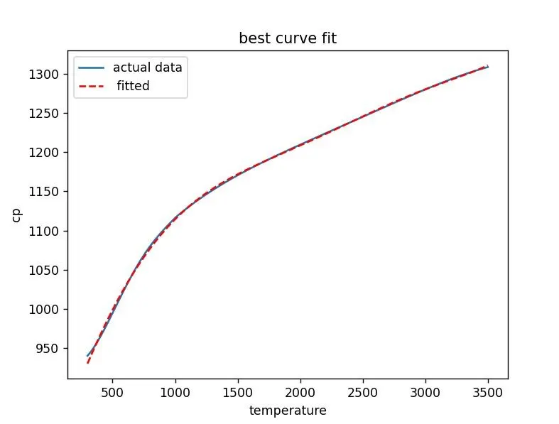
popt,pcov=curve_fit(fun_6,np.array(temp),np.array(cp))
f_6=fun_6(np.array(temp),*popt)
plt.plot(temp,cp)
plt.plot(temp,f_6,"r--")
plt.legend(["actual data"," fitted "])
plt.savefig("forget")
plt.xlabel("temperature")
plt.ylabel("cp")
plt.title("best curve fit")

plt.show()
r_6=f_6 -cp                     #difference between predicted cp and actual cp value
m6=np.array(r_6)
m6=m6*m6                        #squaring the difference values
m6=np.mean(m6)
print(m6,"mean of the squared residuals in polynomial curve fit r_6")
#----------------------------------

Task 5- The methods which we can follow to get the better curve fit are splitting the intervals
where curve fitting is not so proper with the previous curve fitting expression, introducing higher
order polynomial expression to get better fits for the data and we can also introduce
transcendental expression in the expression for better interpretation of the curve fit .
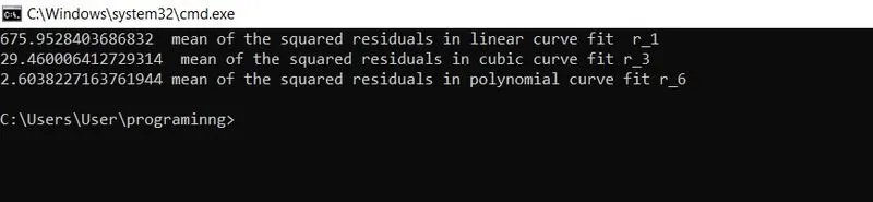
Task 6-To empirically evaluate the curve fits and to compare which one is better we can use the
residuals which is the difference between the predicted output to the actual data ,for better
interpretation we can square the residuals and taking the mean of the data this figure indicates
the better curve fir for the data.m6,m3 and m1 are the mean values for higher order, cubic and
l inear curve fit their order is in the nature of m1>m3>m6.

RESULTS:
The suitable plots and the results displayed in the command prompt are as below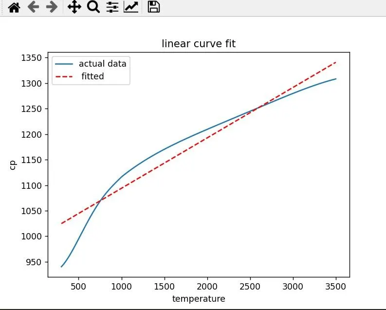

CONCLUSION:
The project has made me understand more about the differences between ND array and list
data format and curve fitting is much more interesting. We can involve higher order polynomial
terms for better approximation of the curve to the given data