Week 3 - Solving second order ODEs
AIM:
Program in Python that will simulate the pendulum motion .
THEORY AND CORRESPONDING EQUATIONS:
The motion of a simple pendulum disturbed which is kept in the surroundings is governed by a second order partial homogeneous linear differential equation which includes its mass,length from the hinge point to the COM ,the gravity due to acceleration and damping constant this system is similar to that of damping system.
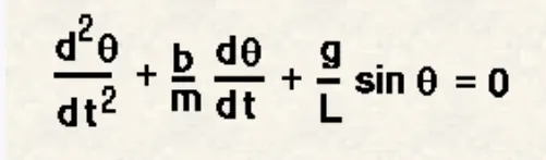
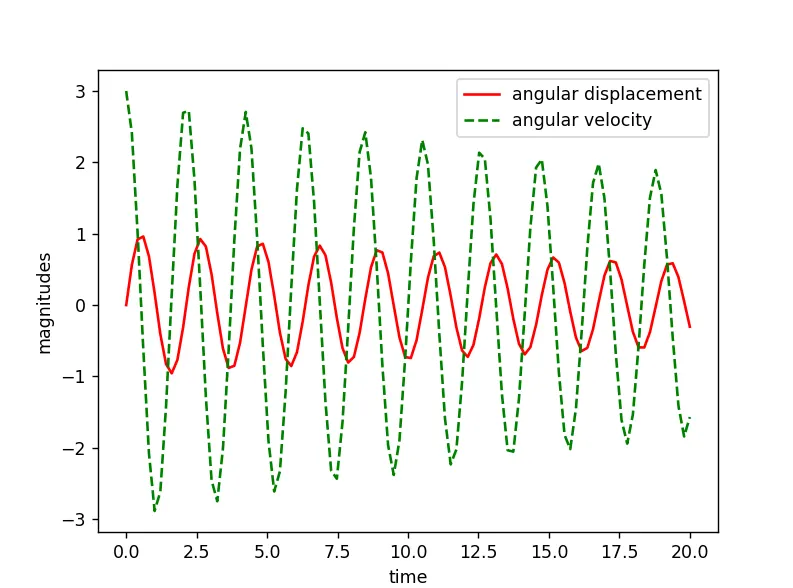
for this simulation I had assumed the initial condition as displacement of the masss to be 0 and the velocity as 3m/s at time 0 apart from given boundary conditions.
x=[L*sin(θ)]
y=[L*cos(θ)]
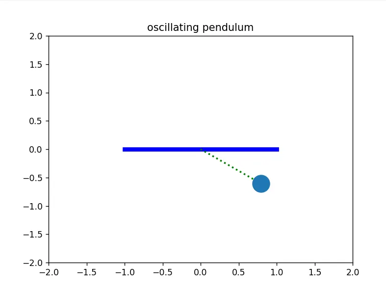
(x and y cordinates made by a pendulum COM of mass m making angle θ with the y axis)
DATA :
L=1 metre,
m=1 kg,
b=0.05.
g=9.81 m/s2.
OBJECTIVE:
The project focuse to solve the ordinary differential equaions with python and the way used to soolve higher order differential equation is to break the equation into several first order differential equations.
BODY OF THE CONTENT:
- Python is used as the programming language
""" program to solve the ordinary differential equations of 2nd order also we will obtain the function of the differential equation and plot the graph with the animation of the pendulum motion. written by GAGAN.k mail id- [email protected] in this program we are going to see how to solve the the differential equation governing the motion of simple pendulum we are going to use odeint from scipy module to integrate this differential equation and ........ to create the animation for the obtained displacement of the simple pendulum. """ #importing suitable libraries for mathematics operation , plotting and integartion operations import math import numpy as np import matplotlib.pyplot as plt from scipy.integrate import odeint """ the pendulum arrangement is taken for understanding differential equation integration in python in this project the equation of motion for the pendulum motion is a second order linear differential ,homogeneous equation this equation is same for damper system arangement from the differential equation of the motion we are going to consider the boundary conditions velocity and displacement at initial time and then integrate for the required time. """ #defining the function for differential equation representation def difeqn(theta,t,b,l,g,m): theta1=theta[0] theta2=theta[1] dtheta1_dt=theta2 dtheta2_dt=(-b/m)*theta2 -(g/l)*math.sin(theta1) dtheta_dt=[dtheta1_dt,dtheta2_dt] return dtheta_dt #inputs for the system b=0.05 #damping coefficient l=1 #length of the COM of the ball from the hinge point(m) g=9.81 #acceleration due to gravity(m/s^2) m=1 #mass of the ball (kg) #initial conditions theta_0=[0,3] #time points t=np.linspace(0,20,100) #solving ode theta=odeint(difeqn,theta_0,t,args=(b,l,g,m)) #plotting result plt.plot(t,theta[:,0],'r-',label="angular displacement") plt.plot(t,theta[:,1],'g--',label="angular velocity") plt.ylabel("magnitudes") plt.xlabel("time") plt.legend() plt.savefig("2ode") plt.show() #animation part ct=1 #creaiing a variable for initialising various filenames for the generated photos x0=0 #cordinates of the hinge point y0=0 #cordinates of the hinge point for angle in theta[:,0]: x=l*math.sin(angle) #cordinates of the COM of the ball attached y=(-1*(l*math.cos(angle))) #cordinates of the COM of the ball attached filename='test%05d.png' % ct #generating filenames ct=ct+1 plt.figure() plt.plot([1,-1],[0,0],"b-",linewidth=5) plt.plot([x0,x],[y0,y],"g:",linewidth=2) plt.plot([x],[y],"o",markersize=20) plt.title('oscillating pendulum') plt.xlim([-2,2]) plt.ylim([-2,2]) plt.savefig(filename) plt.show() - link to acess png and gif files - https://drive.google.com/drive/folders/1BR0wvNKQv_GzbNHBfvvvEqTUah5PlHti?usp=sharing
CONCLUSION:
from this project i got to know about odeint function and got to know how to solve and silmulate some systems which obey differential equation further the assignment will have its value increased if we have a first oder differential equation problem first and then the higher ones .