Week 2 Air standard Cycle

AIM:
Program in python to plot the otto cycle pv plot and find the thermal efficiency of the cycle .

THEORY AND CORRESPONDING EQUATIONS:

thermodynamic specifications-

for any process going from state1 to state2 [control mass]---> ((p1v1)/t1)=((p2v2)/t2)
for isentropic process from state1 to state2 -----> (p1v1^$) = (p2v2^$) [$=(specific heat at constant pressure/specific heat at constant volume)]{which is a constant}
thermal efficiency of the otto cycle is given by -----> 1-(1/(c_r^($-1))) [where c_r is compression ratio defined as the ratio max volume in cylinder to the clearance volume ]

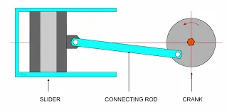
engine specifications-
bore(b) = diameter of the cylinder
swept volume (v_s) = (Pi*(b^2)/4)
compression ratio (c_r) = ratio of max volume in cylinder to the clearance volume
clerance volume (v_c) = v_s/(c_r-1)
volume at salient points in compression and expansion process = product of piston/connecting rod displacement to the stroke length ratio with stroke volume
volume = [v_c+((v_s/sl)*((a+l)-(a*cos(theta))-((l^2) -(a*sin(theta)^2))^0.5))]

OBJECTIVE:

The project focuse on the OTTO cycle thermal efficiency and to plot the corresponding pv plots.

BODY OF THE CONTENT:

Python is used as the programming language

"""
program to simulate the otto cycle and plot the P-V diagram for the same cycle
written by GAGAN.k
mail id- [email protected]
 in this program we are going to see how to plot  the otto cycle pv graph ,we will consider suitable thermal inputs for a 
 spark plug ignition engine which follows otto cycle as a thermodynamic cycle for the energy extraction from fuel like petrol.
 The basics needed for this project is basic kinematics or single crank mechanism features and matplotlib modules .
 
"""

"""
the processes involved in this cycle starts from taking air fuel mixture inside the chamber than next process [1] is 
isentropically compressing the charge till the clearance volume is reached next [2] is constant volume heat addition [3]
is ienstropic expansion followed bby the exhaust at constant volume[4].
"""

#importing suitable  libraries for mathematics operation and plotting operations
import math
import matplotlib.pyplot as plt 

# taking engine cylinder required dimensions honda shine 2 wheeler bike
b=0.05 #bore in m
sl=0.063 #stroke length in m
c_r=9 #compression ration
a=sl/2 #crank pin radius
l=0.15 #connecting_rod_length

#thermal inputs
p1=101325 #atmospheric pressure in pa
t1=400 #average temperature due to heating in the cylinder in k
t3=2000 #maximum temperature the whole cylinder can withstand in k
gamma=1.4 #specific heat ratio

#volume at significant points
v_s=math.pi*math.pow(b,2)*(1/4)*sl #swept volume calculation
v_c=v_s/(c_r-1) #clearance volume
v1=v_s+v_c
v2=v_c
v3=v2
v4=v1

"""volume at the compression and expansion can be find as a part of swept volume by determining 
   the connecting rod displacement"""

#state 1 conditions
p1=101325
v1=v_s+v_c
t1=500
#print(p1,v1,t1)

#state 2 conditions by applying isentropic process between 1 and 2
#p1*v1^gamma=p2*v2^gamma
#for temperature at state 2 ca be obtained by p*v/t=constant
v2=v_c
p2=p1*pow((v1/v2),gamma)
t2=p2*v2*t1/(p1*v1)
g1=p1*pow(v1,gamma)
#print(p2,v2,t2)

#state 3 conditions and using isochoric relation
v3=v2
p3=p2*(v2/v3)*(t3/t2)
g2=p3*(v3)**gamma
#print(p3,v3,t3)

#state 4 conditions using isentropic process conditions
v4=v1
p4=p3*pow((v3/v4),gamma)
t4=p4*v4*t3/(p3*v3)
#print(p4,v4,t4)
#calculating volume and pressure at intermediate points at compression and expansion process
def volume_cal(strt_angle,end_angle):
	V=[]
	steps=100
	c1=a+l#constant 1
	dtheta=(end_angle-strt_angle)/(steps-1)
	
	for i in range(0,steps):
		theta=math.radians(strt_angle+(i*dtheta))
		#print(theta)
		
		
		n=(l**2)-((a*math.sin(theta))**2) #constant 
		#print(c3)
		j=v_c+((v_s/sl)*((a+l)-(a*math.cos(theta))-pow(n,0.5)))

		V.append(j)
	return V

def pressure_cal(v,g):
	p=[]
	for i in range(len(v)):
		t=g/(v[i]**gamma)
		p.append(t)

	return p



v_expansion=volume_cal(0,180)
p_expansion=pressure_cal(v_expansion,g1)
v_compression=volume_cal(180,0)
p_compression=pressure_cal(v_compression,g2)



#calculating thermal efficiency of the otto cycle (nt)
nt=1-(1/(c_r**(gamma-1)))
print("efficiency of the cycle is ",nt*100,"%")

#plotting the graph
plt.title(" OTTO CYCLE P vs V")
plt.xlabel("volume")
plt.ylabel("pressure")
plt.plot([v2,v3],[p2,p3])
plt.plot(v_compression,p_compression)
plt.plot(v_expansion,p_expansion)
plt.plot([v4,v1],[p4,p1])
plt.savefig("otto")
plt.show()

RESULTS:

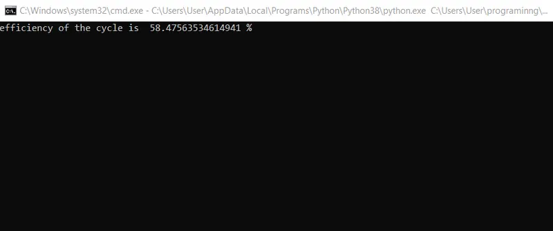
Screenshot showing the thermal efficiency output

plot of the P vs V of otto cycle

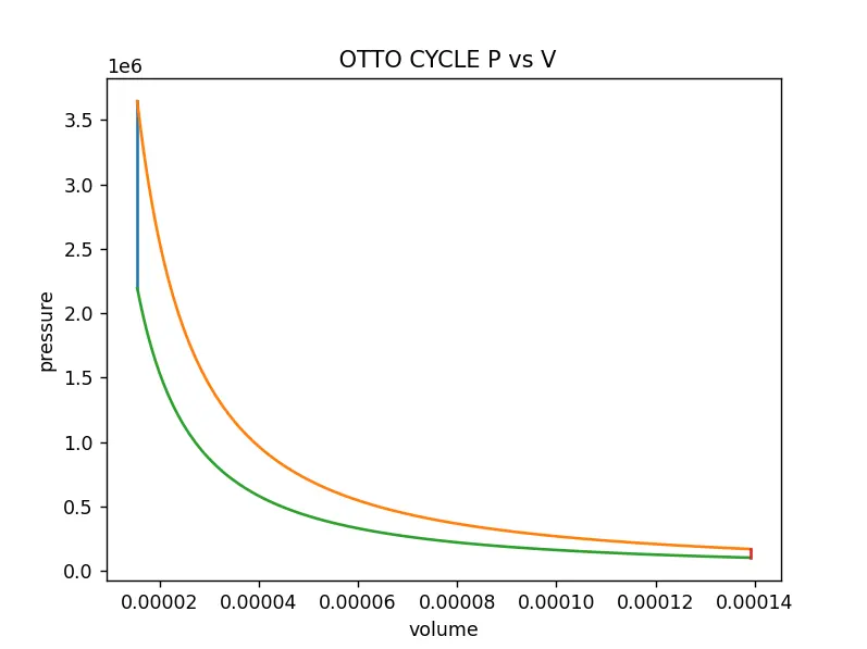
COCLUSION:

The theramal efficiency of the otto cycle for assumed thermal conditions is found to be 58.47563534614941 % and plot of the pv graph is obtained similar to that of ideal one.