Week 5 - Curve fitting

CURVE FIT

1. What does popt and pcov mean? (Watch the video to get some context)

Ans: The popt argument contains best fit parameters for the variables a and b

The pcov variable contains the covariance matrix, which indicates the uncertainties and correlations between parameters. This is mostly useful when the data has uncertainties.

2. What does np.array(temperature) do?

Ans: The command 'np.array(temparature)' is used for accessing the inividual elements of the temperature array with the help of numpy module.

3. What does the * in *popt mean?

Ans: It referring to all the values stored in the array 'popt'.

4. Write code to fit a linear and cubic polynomial for the Cp data. Explain if your results are good or bad.

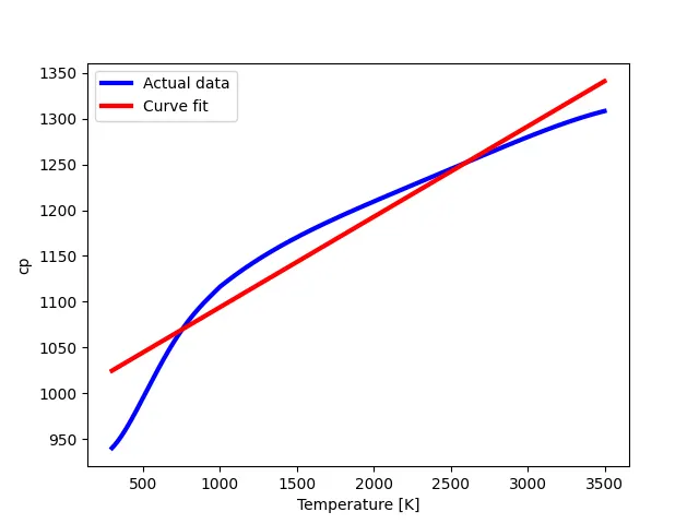
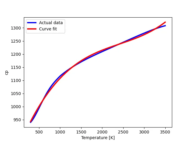
Ans: The code linear and cubic polynomial for the cp data below it shows that the linear curve has the large deviations and the cubic curve gives better fit to with small deviation

5. What needs to be done in order to make the curve fit perfect?

Ans:'popt' (best fit value of coefficients) and 'pcov' (estimated value of covariance of coefficients) should use for curve fit perfect.

6. Show empirically as to how well your curve has been fit.

Ans: Empirically it shows that cubic curve has less deviation and perfect fit compared to linear one

Code explination

• Initially import the useful libraries like math, matplotlib, numpy and curve_fit form scipy_optimize
• defining function for linear equation
• defining function for cubic equation
• code to read the given data files for temparature and cp values
• after that call curve fit library with popt and pcov to genarate curve fit for linear equation
• The above step is repeat for cubic equation
• Then compare the deviation achived between linear eq and cubic eq for given data
• Then conclude the obtained result

import math
import numpy as np
import matplotlib.pyplot as plt
from scipy.optimize import curve_fit 

#curve fit function

#Linear Polynomial
def func1(t, a, b):
	return a*t + b
#Cubic polynomial
def func2(t, a, b, c, d):
	return a*(t**3) + b*(t**2) + c*t + d 

#To read thermodynamic data file 
def read_file():
	temperature = []
	cp = []
	for line in open('data','r'):
		values = line.split(',')
		temperature.append(float(values[0]))
		cp.append(float(values[1]))

	return [temperature, cp]

#Linear fit
temperature, cp = read_file()
popt, pcov = curve_fit(func1, temperature, cp)
fit_cp = func1(np.array(temperature), *popt)

plt.plot(temperature, cp,, linewidth=3)
plt.plot(temperature, fit_cp,, linewidth=3)
plt.legend(['Actual data','Curve fit'])
plt.xlabel('Temperature [K]')
plt.ylabel('cp')
plt.savefig('Linear_fit'+'.png')
plt.show()

#Cubic fit
temperature, cp = read_file()
popt, pcov = curve_fit(func2, temperature, cp)
fit_cp = func2(np.array(temperature), *popt)

plt.plot(temperature, cp,, linewidth=3)
plt.plot(temperature, fit_cp,, linewidth=3)
plt.legend(['Actual data','Curve fit'])
plt.xlabel('Temperature [K]')
plt.ylabel('cp')
plt.savefig('Curve_fit'+'.png')
plt.show()

Linear equation curve fit

Using liner equation the plot is not so satisfying because it has lot of variation in comparision to actual curve so the results are bad for linear equation

Cubic equation curve fit

By using cubic polynomial it has a less difference in the polt so the variation less so the result is good for this cubic equation

Conclusion

In above cuve fit there is some error in cubic equation also so, In order to make the curve fit perfect error estimation should also be considered