Week 5 - Curve fitting
- What does popt and pcov mean? (Watch the video to get some context)
-->
“popt” = It contains optimal values for the model function(optimal coefficient values of the polynomial). Internally contains fit results for the slope and fit results for intercept.
“pcov” = The pcov variable contains the covariance matrix, which indicates the uncertainties and correlations between parameters. This is mostly useful when the data has uncertainties
- What does np.array(temperature) do?
-->
Using np.array(temperature), all temperature values are passed as an array, so that the function returns solution in an array form.
- What does the * in *popt mean?
-->
* means all. Since popt contains optimal value of various coefficients, *popt allows to extract all values of the coefficients.
- Write code to fit a linear and cubic polynomial for the Cp data. Explain if your results are good or bad.
-->
Procedure:
- Load necessary modules such as numpy, matplotlib, scipy, and statistics.
- First case is curve fitting using Linear polynomial, so define a function to solve the linear polynomial.
- Define a function to read the ‘data’ file and extract the values into arrays.
- Use “curve_fit” function to get optimal coefficient values of the linear polynomial.
- Pass these optimal coefficient values into the function and solve for predicted results.
- Plot the comparison curves between actual data and the predicted data.
- Calculate the goodness of fit using R square method and display if curve is good fit or bad fit.
- Second case is curve fitting using Cubic polynomial, so define a function to solve the cubic polynomial.
- Follow the same process as done for curve fitting using linear polynomial. Plot the comparison curves and display if curve is good fit or bad fit.
Code:
"""
Curve Fitting
"""

# Linear polynomial Curve fit

import numpy as np
import matplotlib.pyplot as plt
from scipy.optimize import curve_fit
from statistics import mean

# Curve fit function(1nd order-linear polynomial)

def func(t,a,b):
	return a*t + b

# reading thermodynamic data file

def read_file():
	temperature = []
	cp = []
	for line in open('data','r'):
		values = line.split(',')
		temperature.append(float(values[0]))
		cp.append(float(values[1]))

	return [temperature,cp]

# main program

temperature,cp = read_file()
popt,pcov = curve_fit(func,temperature,cp)
fit_cp = func(np.array(temperature),*popt)

# plotting
plt.figure(0)
plt.plot(temperature,cp,color='b',linewidth=3)
plt.plot(temperature,fit_cp,color='r',linewidth=3)
plt.legend(['Actual data','Linear polynomial curve fit'])
plt.xlabel('Temperature[k]')
plt.ylabel('Cp')
plt.title('Comparision plot of Actual data and Predicted data')
plt.show()

# Goodness of fit

error = fit_cp-cp
SSE = sum(error*error)
SSR = sum(pow(fit_cp-mean(fit_cp),2))
SST = SSR +SSE
R_Square = SSR/SST
print("R Square value of curve fit using linear polynomial: ",R_Square)

if (R_Square==1):
	print("Best fit")
elif (R_Square>0.95):
	print("Good fit")
else:
	print("Bad fit")
print("\n")

# Cubic polynomial Curve fit
# Curve fit function(3rd order-cubic polynomial)

def func(t,a,b,c,d):
	return a*pow(t,3) + b*pow(t,2) + c*t + d

# reading thermodynamic data file

def read_file():
	temperature = []
	cp = []
	for line in open('data','r'):
		values = line.split(',')
		temperature.append(float(values[0]))
		cp.append(float(values[1]))

	return [temperature,cp]

# main program

temperature,cp = read_file()
popt,pcov = curve_fit(func,temperature,cp)
fit_cp = func(np.array(temperature),*popt)

# plotting
plt.figure(1)
plt.plot(temperature,cp,color='b',linewidth=3)
plt.plot(temperature,fit_cp,color='r',linewidth=3)
plt.legend(['Actual data','Cubic polynomial curve fit'])
plt.title('Comparision plot of Actual data and Predicted data')
plt.xlabel('Temperature[k]')
plt.ylabel('Cp')
plt.show()

# Goodness of fit

error = fit_cp-cp
SSE = sum(error*error)
SSR = sum(pow(fit_cp-mean(fit_cp),2))
SST = SSR +SSE
R_Square = SSR/SST
print("R Square value of curve fit using cubic polynomial: ",R_Square)


if (R_Square==1):
	print("Best fit")
elif (R_Square>0.95):
	print("Good fit")
else:
	print("Bad fit")

print("\n")
Result explaination:
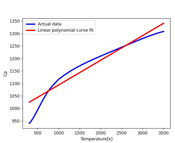
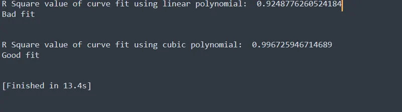
Using "Linear polynomial" for curve fitting, R Square value obtained was 0.9248. If R Square value is less than 0.95, it is considered as a “Bad fit”.
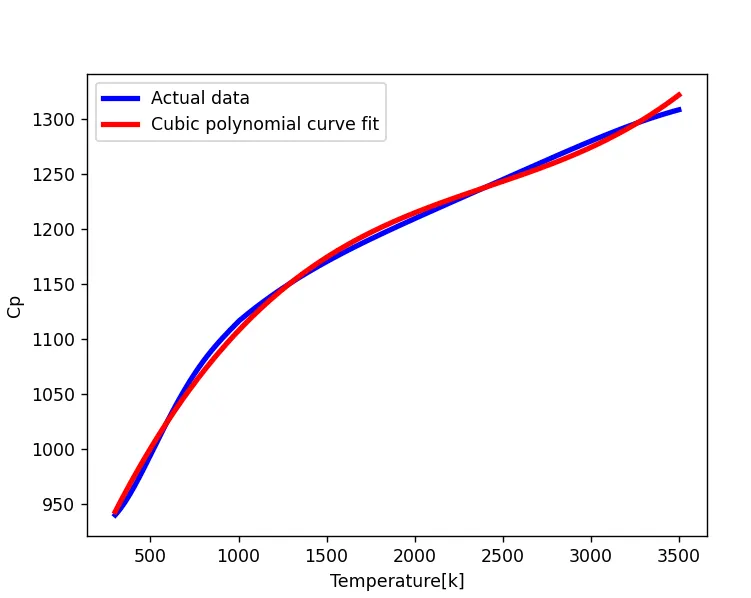
Using "Cubic polynomial" for curve fitting, R Square value obtained was 0.9967. If R Square value is greater than 0.95, it is considered to be a “Good fit”.
- What needs to be done in order to make the curve fit perfect?
-->
To make a curve fit perfectly we can increase the order of polynomial or we can use “Split wise” method where the data set is broken into fragments and the matching equation is obtained for the fragmented data set.
- Show empirically as to how well your curve has been fit.
-->
Results:
- Below figure shows the comparision plot between actual data and predicted data solved using Linear polynomial. The curve obtained using the predicted data intersects the curve with actual data at few points but still the deviation(error) is large. When calculated the goodness of fit using R square method, the R square value was found to be 0.9248, which is considered to be bad fit as it is less than 0.95.
- Below figure shows the comparision plot between actual data and predicted data solved using Cubic polynomial. The curve obtained using the predicted data overlapse the curve with actual data for most of the part. When calculated the goodness of fit using R square method, the R square value was found to be 0.9967, which is considered to be good fit as it is greater than 0.95.
- Below figure shows the output window displaying the R square values and Goodness of fit obtained using linear polynomial and cubic polynomial respectively. Using linear polynomial for curve fitting, we get bad fit and using cubic polynomial for curve fit we get good fit.
Discussion: The plots are generated for curve fit using linear and cubic polynomial where we got bad curve fit using linear polynomial and good curve fit using the cubic polynomial. As we increase the order of polynomial we get better fit, but if we keep increasing order of polynomial, after certain limit "overfitting" occurs where model begins to describe random error.
References: