Challenge

Project 2 - Rankine cycle Simulator

SSuraj Dhavaleshwar13 Nov 2021

MATLAB

RANKINE CYCLE SIMULATOR

XSteam library:- https://drive.google.com/file/d/1RK_fvrOj38CIaQvmLT1S3daqHnxKCGU-/view?usp=sharing

AIM: To create Rankine cycle simulator

OBJECTIVE:

To calculate the state points of the Rankine cycle
Plot T-S and H-S plots for given set of inputs

BODY OF CONTENT:

Programming language: MATLAB

Code:

% Rankine Cycle Simulator

clear all
close all
clc
%%
% T     Temperature (deg C)
% p	    Pressure    (bar)
% h	    Enthalpy    (kJ/kg)
% v	    Specific volume (m3/kg)
% rho	Density
% s	    Specific entropy 
% u	    Specific internal energy 
% Cp	Specific isobaric heat capacity 
% Cv	Specific isochoric heat capacity 
% x	    Vapour fraction
% Wp    Work by compressor   
% Wt    Work by turbine
% Wnet  Net work done
% Ntherm Thermal efficiency
% SSC   Specific steam consumption
%%

% User inputs

fprintf('\n RANKINE CYCLE SIMULATOR');
fprintf('\n\n1-2 is a Isentropic Expansion in the Turbine');
fprintf('\n2-3 is a Constant Pressure Heat Rejection by the Condenser');
fprintf('\n3-4 is a Isentropic Compression in the Pump');
fprintf('\n4-1 is a Constant Pressure Heat  Addition by the Boiler\n');
p1 = input('\nEnter the Pressure at the Turbine Inlet (in bar): ');
t1 = input('Enter the Temperature at the Turbine Inlet (in Degree Celcius): ');
p2 = input('Enter the Pressure at the Condenser (in bar): ');

% Calculations
p3 = p2;
p4 = p1;
h3 = XSteam('hL_p',p3);
s3 = XSteam('sL_p',p3);
v3 = XSteam('vL_p',p3);
t3 = XSteam('Tsat_p',p3);
t2 = t3;
s4 = s3;
cp4 = XSteam('Cp_ps',p4,s4);
cv4 = XSteam('Cv_ps',p4,s4);
g4 = cp4/cv4;
o = (g4-1)/g4;
t4 = t3*((p4/p3)^o);
Wp = v3*(p4-p3)*100;
h4 = h3+Wp;
h1 = XSteam('h_pT',p1,t1);
s1 = XSteam('s_pT',p1,t1);
s2 = s1;
sf2 = XSteam('sL_p',p2);
sg2 = XSteam('sV_p',p2);
hf2 = XSteam('hL_p',p2);
hg2 = XSteam('hV_p',p2);
x2 = ((s2-sf2)/(sg2-sf2));
h2 = hf2+(x2*(hg2-hf2));
p5 = p4;
t5 = XSteam('Tsat_p',p5);
h5 = XSteam('hL_T',t5);
s5 = XSteam('sL_p',p5);
t6 = t5;
p6 = XSteam('psat_T',t5);
s6 = XSteam('sV_T',t6);
h6 = XSteam('hV_T',t6);

Wt = h1-h2;                 % Work done by turbine
Wnet = Wt-Wp;               % Net work done
Qin = h1-h4;                % Heat addition
Qout = h2-h3;               % Heat rejection
Ntherm = Wnet/Qin;          % Thermal efficiency
BWR = Wp/Wt;                % Back work ratio
SSC = 3600/Wnet;            % Specific steam consumption

fprintf('\nAt State point 1:\n');
fprintf('\nP1 is : %f Bar',p1);
fprintf('\nT1 is : %f Deg Celcius',t1);
fprintf('\nH1 is : %f kJ/kg',h1);
fprintf('\nS1 is : %f kJ/kgK',s1);

fprintf('\n\nAt State point 2:\n');
fprintf('\nP2 is : %f Bar',p2);
fprintf('\nT2 is : %f Deg Celcius',t2);
fprintf('\nH2 is : %f kJ/kg',h2);
fprintf('\nS2 is : %f kJ/kgK',s2);
fprintf('\nX2 is : %f',x2);

fprintf('\n\nAt State point 3:\n');
fprintf('\nP3 is : %f Bar',p3);
fprintf('\nT3 is : %f Deg Celcius',t3);
fprintf('\nH3 is : %f kJ/kg',h3);
fprintf('\nS3 is : %f kJ/kgK',s3);

fprintf('\n\nAt State point 4:\n');
fprintf('\nP4 is : %f Bar',p4);
fprintf('\nT4 is : %f Deg Celcius',t4);
fprintf('\nH4 is : %f kJ/kg',h4);
fprintf('\nS4 is : %f kJ/kgK',s4);

fprintf('\n\nAt State point 5:\n');
fprintf('\nP5 is : %f Bar',p5);
fprintf('\nT5 is : %f Deg Celcius',t5);
fprintf('\nH5 is : %f kJ/kg',h5);
fprintf('\nS5 is : %f kJ/kgK',s5);

fprintf('\n\nAt State point 6:\n');
fprintf('\nP6 is : %f Bar',p6);
fprintf('\nT6 is : %f Deg Celcius',t6);
fprintf('\nH6 is : %f kJ/kg',h6);
fprintf('\nS6 is : %f kJ/kgK',s6);

fprintf('\n\nWt is : %f kJ/kg',Wt);
fprintf('\nWp is : %f kJ/kg',Wp);
fprintf('\nWnet is : %f kJ/kg',Wnet);
fprintf('\nBWR is : %f',BWR);
fprintf('\nNtherm is : %f Percent',Ntherm);
fprintf('\nSSC is : %f kg/kWh\n',SSC);

% using for loop to obtain points for Liquid and Vapour lines
t = linspace(0,400,1000);
for i = 1:length(t)
    S_l1(i) = XSteam('sL_T',t(i));
    S_l2(i) = XSteam('sV_T',t(i));
    H_l1(i) = XSteam('hL_T',t(i));
    H_l2(i) = XSteam('hV_T',t(i));
end

% Plotting T-S and H-S 
figure(1)
hold on
plot([S_l1 S_l2],[t t],'color','b','linewidth',2)
plot([s1 s2 s3 s4 s5 s6 s1],[t1 t2 t3 t4 t5 t6 t1],'color','r','linewidth',2)
text(s1,t1,'1')
text(s2,t2,'2')
text(s3,t3,'3')
text(s4,t4,'4')
text(s5,t5,'5')
text(s6,t6,'6')
title('T-S Diagram')
xlabel('Entropy (kJ/kgK)')
ylabel('Temperature (Deg Celcius)')
axis([0,8,0,450])

 
figure(2)
hold on
plot([S_l1 S_l2],[H_l1 H_l2],'color','b','linewidth',2)
plot([s1 s2 s3 s4 s5 s6 s1],[h1 h2 h3 h4 h5 h6 h1],'color','r','linewidth',2)
text(s1,h1,'1')
text(s2,h2,'2')
text(s3,h3,'3')
text(s4,h4,'4')
text(s5,h5,'5')
text(s6,h6,'6')
title('H-S Diagram')
xlabel('Entropy (kJ/kgK)')
ylabel('Enthalpy (kJ/kg)')
axis([0,8,0,3500])

EXPLAINATION:

Initially the input parameters such as Turbine inlet pressure, Turbine inlet temperature and Condenser pressure which are state point variables are initialized by user inputs
Then the remaining state points variables are calculated and XSteam library function is used to get some required parameters
Work at turbine, Work at compressor, Net work done, Heat in, Heat out, Thermal efficiency, Back work ratio and Specific steam consumption are calculated
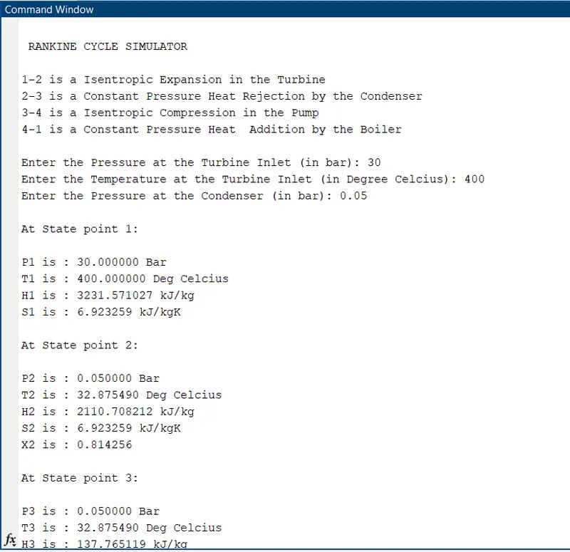
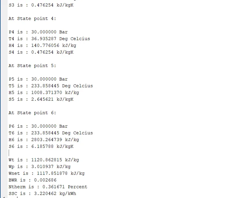
All the state point variables are displayed in the command window along with the calculated Work at turbine, Work at compressor, Net work done, Heat in, Heat out, Thermal efficiency, Back work ratio and Specific steam consumption
The points to create the liquid and vapour lines are generated using the for loop
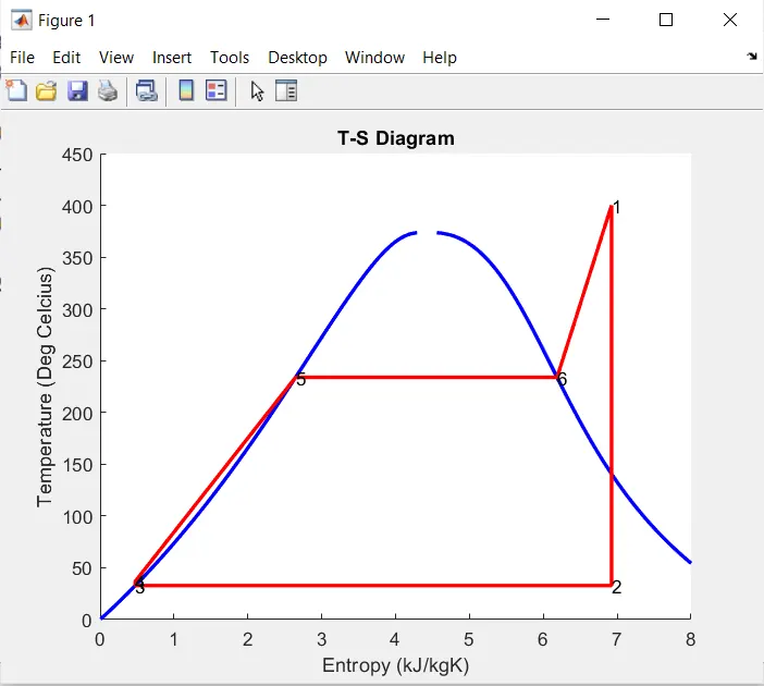
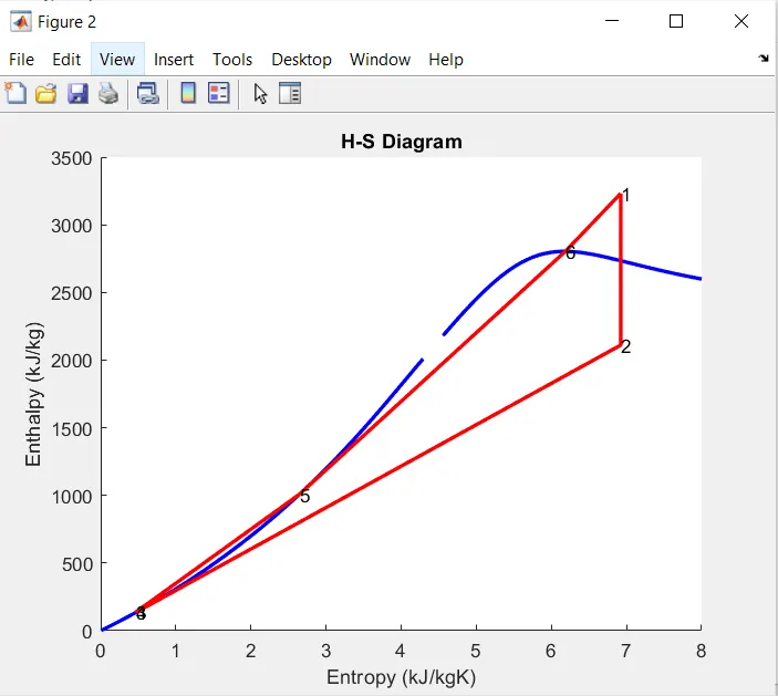
Temperature vs Entropy and Enthalpy vs Entropy plots are plotted

OUTPUT:

Command window output showing the state point variables

T_S diagram of Rankine cycle

H-S diagram of Rankine cycle

CONCLUSION: Concept of Rankine cycle is understood and the code for simulating the same has been created and the state point variables are displayed and the plots of Temperature vs Entropy and Enthalpy vs Entropy has been plotted. With this code with the user inputs of Turbine inlet pressure, Turbine inlet temperature and Condenser pressure the Rankine cycle plots and state point variables can be extracted

REFERENCES:

Project 2 - Rankine cycle Simulator

Ship work like this
in your own course.

Talk to a career counsellor

Ship work like thisin your own course.

Talk to a career counsellor

Ship work like this
in your own course.