Week 3 - Solving second order ODEs

Animation of Simple Pendulum Motion

1. AIM: To simulate the simple pendulum motion with damper

2. EQUATION:

`(d^2 θ)/(dt^2 )+b/m (dθ)/(dt)+g/L sin⁡θ=0`

Where,

b = damping coefficient

m = mass of the ball, kg

g = gravity, m/s²

L = length of the pendulum, m

• Simple pendulum motion depends on Newton’s second law, which says ‘Total force being applied to a moving body represents the motion of the body’
• The key factor in this governing equation is Torque, and it comes from gravity, since no additional force is applied to pendulum
• Here the governing equation is of second order ODE, to solve this differential equation we use ode45 solver, which is an inbuilt MATLAB function
• But for ode45 to work, we must break original second order ODE into two first order ODE’s
• Then these first order ODEs are stored in matrix form and then ode45 can solve this and provide solution results

3. OBJECTIVES:

• To write a program that solves ordinary differential equation
• Create an animation showing the motion of pendulum

4. BODY OF CONTENT:

Code

% Program to simulate the simple pendulum motion 

clear all 
close all
clc

% Given Inputs
b = 0.05;       % damping coefficient
g = 9.81;       % gravity, m/s^2
l = 1;          % length of the pendulum, m
m = 1;          % mass of the ball, kg

% Initial conditions( Angular Displacement, Angular Velocity)
theta_0 = [0,3];

% Time points 
t_span = linspace(0,20,500);

% Solving ODE
[t, results] = ode45(@(t,theta) ode_func(t,theta,b,g,l,m),t_span,theta_0);

% Plotting results
figure(1)
plot(t,results(:,1))
hold on
plot(t,results(:,2))
xlabel('Time')
ylabel('Angular Displacement and Angular Velocity')
legend('Angular Displacement','Angular Velocity')
hold off

% Counter (ct)
ct = 1;

% using 'for' loop to change theta1(Angular displacement) values automatically 
% i is loop counter variable
for i = 1:length(results(:,1))
    % Coordinates of pendulum start and end points (x0,y0),(x1,y1)
    x0 = 0;
    y0 = 0;
    
    x1 = l*sin(results(i,1));
    y1 =-l*cos(results(i,1));

    
% Plotting 

figure(2)

plot([-1 1], [0 0], 'linewidth',3,'color','r')
hold on
plot([x0 x1],[y0 y1],'linewidth',2,'color','g')

title('Pendulum motion simulation')
xlabel('x-axis')
ylabel('y-axis')

plot(x0,y0,'marker', 'o','MarkerSize',7 ,'MarkerFaceColor','k')
plot(x1,y1,'marker', 'o','MarkerSize',20 ,'MarkerFaceColor','b')
axis( [-1.5 1.5 -1.5 0.5])
hold off
pause(0.05)

% 'M' is an array used to store individual frames, and here 'ct' represents individual frame
M(ct) = getframe(gcf);

ct = ct+1;

end

% Creating movie
movie(M)
% Creating avi file to store all frames
videofile = VideoWriter('pendulum_simulation.avi','Uncompressed AVI');
open(videofile)
% Creating video using frames
writeVideo(videofile,M)
close(videofile)

function code

% function defination for solving second order ode
function [dtheta_dt] = ode_func(t,theta,b,g,l,m)

theta1 = theta(1);
theta2 = theta(2);
dtheta1_dt = theta2;
dtheta2_dt = -(b/m)*theta2-(g/l)*sin(theta1);
dtheta_dt = [dtheta1_dt;dtheta2_dt];

end

Code explanation

• Initially defining the given inputs such as damping coefficient(b), gravity(g), length of pendulum(L), mass of the ball(m) and Initial conditions such as of angular displacement and angular velocity
• Then we define time span, which gives the range to integrate the differential equation with provided initial conditions
• Then we use ode45 function to solve the differential equation, in which we make a function call of the function named ode_func and obtain the solution results
• This function template ode_func gives values of angular displacement and angular velocity for the given time span
• Syntax of ode45:

[TOUT, YOUT] = ode45(ODEFUN, TSPAN, Y0)

Where,

TOUT, YOUT are outputs

Ode45 is a function which is used to solve differential equations

ODEFUN is a function handle

TSPAN is a vector with several time points

Y0 is a column vector with initial conditions

• Next, we plot the solution results, showing the wave curves of angular displacement and angular velocity against time
• And then we plot another series of figures using the ‘for loop’ for the purpose of animation of pendulum motion
• Then all the figures are stored in an array M, and then using movie command, the movie is created using these figures
• Then using ‘video writer’ command, the video file name and file type are defined, and the movie is stored in that file.

5. ERRORS:

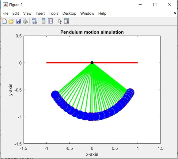
• I got this error where all the figures were overlapping, when I debugged the code I got to know that I was missing the hold off command after line 60, since we used hold on command due to multiple use of plot command and these plots are inside for loop, we must use hold off command to stop overlapping of figures

6. OUTPUTS:

• Angular displacement and Angular Velocity against time plot

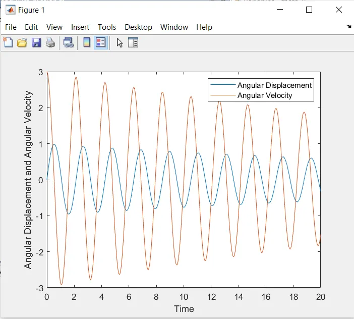
From above plot we can observe that the angular displacement and angular velocity values are damping out and after some time these values are going to equal to zero and the waves will get flat

• Animation of the simple pendulum motion

Youtube link:

https://youtu.be/u8mkPXZx6_A

The above video shows the animation of simple pendulum motion which was created in matlab by solving the governing equation of motion which is second order ODE, and the function ode45 id used to solve it and the solutions were plotted and movie was made using the figures. We can see that the video is about 17 seconds and the pendulum is slowing down with time as the damping effect is considered in the program, which means after some time the pendulum will stop oscillating

7. CONCLUSION:

The graph of Angular velocity and Angular displacement against time has been plotted, and we can see the damping effect as the values of angular displacement and angular velocity keeps decreasing. We have also created a animation movie showing the simple pendulum motion, from which we can observe that oscillation is decreasing and the back and forth motion slowing down over time. In this program we learnt solving the second order ODE using ode45 function and creating an animation using movie command