Week 5 - Curve fitting

Curve Fitting

Aim- To study curve fitting

Objectives-

1) To study curve fitting

2) To find correlation constsnts of given data

Answers to questions

Ans.1 popt is representing values of a,b,c,d and pcov represents coefficient of regression

Ans.2 np.temperature() is passing entire temperature array for curve fitting

Ans.3 Code-

#importing required modules
import math
import numpy as np
import matplotlib.pyplot as plt
from scipy.optimize import curve_fit
#defining function for cubic polynomial
def temp1(t,a,b,c,d):
	return a*pow(t,3)+b*pow(t,2)+c*t+d
def temp2(t,a,b):
	return a*t+b
#defining function to raed the data(cubic)
def readfile():
	t=[]
	cp=[]
	for l in open('data','r'):
		values=l.split(',')
		t.append(float(values[0]))
		cp.append(float(values[1]))
	return(t,cp)
t,cp=readfile()
# finding all constants (cubic)
popt,pcov=curve_fit(temp1,t,cp)
# finding all constants (linear)
pop,pco=curve_fit(temp2,t,cp)
# curve fitting(cubuc)
fit_cp1=temp1(np.array(t),*popt)
# curve fitting(linear)
fit_cp2=temp2(np.array(t),*pop)
#Plotting the fitted curve(cubic)
plt.plot(t,cp,color="red",linewidth=2)
plt.plot(t,fit_cp1,color="green",linewidth=2)
plt.legend(['Actual Data','Curve Fit'])
plt.xlabel('Temperature')
plt.ylabel('Specific Heat')
#Plotting the fitted curve(linear)
plt.plot(t,cp,color="blue",linewidth=2)
plt.plot(t,fit_cp2,color="black",linewidth=2)
plt.legend(['Actual Data','Curve Fit'])
plt.xlabel('Temperature')
plt.ylabel('Specific Heat')
plt.show()

Result

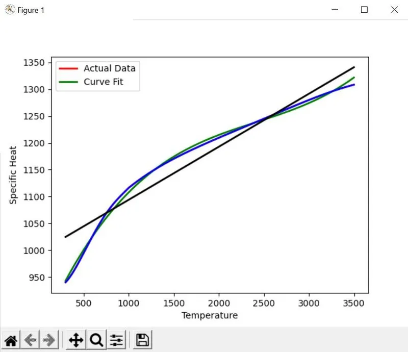
Ans 4. Results of curve fit with cubic polynomial is good but result of linear polynomial is poor

Ans 5. We can use higer degree polynomial to improve curve fitting

Ans 6. As we go from linear to cubic curve fitting becames near to the perfect

Conclusion-

Successfully studied curve fitting