Week 3 - Solving second order ODEs

Simple Pendulum

Aim- To study simple pendulum

Objective-

• To study simple pendulum
• To write program in python to solve second order differential equation
• To write program in python to get velocity and displacement
• To upload animation video of simple pendulum on YouTube

Theory-

In simple pendulum mass is suspended from pivot by using thread. If we give initial displacement or initial velocity to mass pendulum starts oscillating. If there is no air resistance to oppose pendulum motion pendulum keep on oscillating for unlimited time. If there is air resistance that means damping resistance pendulum oscillates but its amplitude and velocity goes on decreasing.

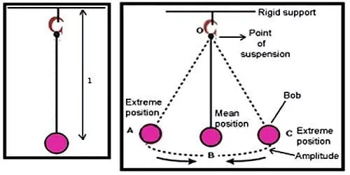
Fig. Simple Pendulum[1]

Problem Statement-

Simulate the motion between 0-20 sec, for angular displacement=0,angular velocity=3 rad/sec at time t=0.

Calculation-

The equation for simple pendulum is given as,

d²ϴ/dt²+b/m dϴ/dt+g/L sinϴ

g = gravity in m/s2,

L = length of the pendulum in m,

m = mass of the ball in kg,

b=damping coefficient.

Write a program in Python that will simulate the pendulum motion, just like the one shown in the start of this challenge.

use,

L=1 metre,

m=1 kg,

b=0.05.

g=9.81 m/s2.

# importing required modules
import math
import numpy as np
import matplotlib.pyplot as plt
from scipy.integrate import odeint
# defining variables
l=1
g=9.81
#defining function to plot output of ODE
def model(theta,t,b,g,l,m):
	theta1 = theta[0]
	theta2 = theta[1]
	dtheta1_dt=theta2
	dtheta2_dt=-b/m*theta2-g/l*math.sin(theta1)
	dtheta_dt=[dtheta1_dt,dtheta2_dt]
	return dtheta_dt
theta_0=[0,3]
t = np.linspace(0,20,100)
theta=odeint(model,theta_0,t,args=(0.05,g,l,1))
plt.plot(t,theta[:,0],'b-',label=r'$\frac{d\theta_1}{dt}=\theta2$')
plt.plot(t,theta[:,1],'r--',label=r'$\frac{d\theta_2}{dt}=-\frac{b}{m}\theta_2-\frac{g}{l}sin\theta_1$')
plt.ylabel('Plot')
plt.xlabel('Time')
plt.legend(loc='best')
plt.show()
# Definibg function for simulation
g=theta[:,0]
no_of_frames=1
for ang in g:
	x0=0
	y0=0
	x1=-l*math.sin(ang)
	y1=-l*math.cos(ang)
	filename='pend%05d.png'%no_of_frames
	plt.figure()
	plt.plot([-1,1],[0,0],linewidth=3)
	plt.plot(x1,y1,'o',markersize=12)
	plt.xlim([-1.5,1.5])
	plt.ylim([-1.5,1.5])
	plt.savefig(filename)
	no_of_frames=no_of_frames+1

Explanation-

• Imported math module for calculation
• Imported matplotlib model for plotting velocities and displacement
• Defined function to solve second order differential equation
• Defined integration limits
• Defined pendulum parameters i.e. length, mass, damping coefficient etc.
• Called function for getting plot
• Plotted velocities and displacements using plt.
• Function Defined for simulation
• Got images of different position of pendulum
• Made animated video
• Uploaded on You Tube

Result-

• Plot of velocities and displacements

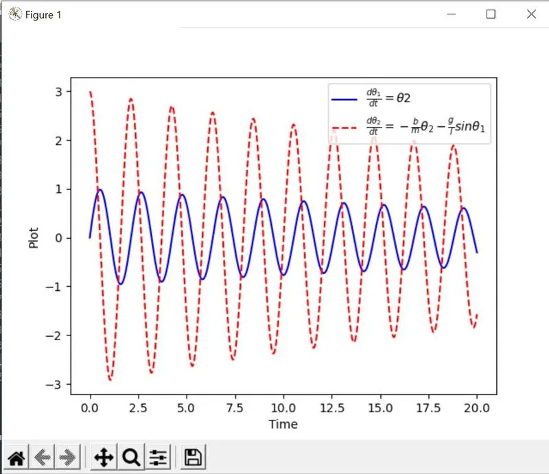
2) You Tube Link

https://youtu.be/3UjPV6zhyac

Conclusion-

Successfully plotted velocities and displacements for simple pendulum

Successfully Uploaded simulation video on You Tube

References-

[1] https://www.google.com/url?sa=i&url=https%3A%2F%2Fqsstudy.com%2Fphysics%2Fthe-laws-of-a-simple-pendulum&psig=AOvVaw0z7lMXBTQUnCTTt0KFgjPz&ust=1634194738752000&source=images&cd=vfe&ved=0CAsQjRxqFwoTCNCr2vrnxvMCFQAAAAAdAAAAABAD