Week 5 - Curve fitting

Introduction:

Curve fitting is the process of specifying the model that provides the best fit to the specific curves in the dataset. Curve fitting can involve either interpolation where an exact fit to the data is required, or smoothing in which a "smooth" function is constructed that approximately fits the data. In this challenge, a curve fit for the variation of specific heat with temperature is done using python software.

Objectives:

To find the best curve fit for the variation of specific heat with the temperature.

What does popt and pcov mean?

popt returns the optimal values for the parameters so that the sum of the squared residuals for the f(x) in this case specific heat is minimized.

pcov returns estimated covariance of popt. The diagonal of the matrix provides the variance of the parameter estimate.

Popt pcov values for the linear function

popt=[9.87543761e-02 ,9.95201748e+02]
pcov=[[ 2.47696157e-07 -4.70498850e-04]
[-4.70498850e-04 1.10507993e+00]]

What does np.array(temperature) do?

np represents 'numpy' which performs array operations. np. array(temperature) collects the temperature values from the data and stores it as an array(collection of numbers and save it in a single variable).

What does the * in *popt mean?

*args in function definitions in python is used to pass a variable number of arguments to a function. In this challenge, the *popt sends the coefficient values a,b and c to the function to calculate updated specific heat values ie fit_cp

Write code to fit a linear and cubic polynomial for the Cp data. Explain if your results are good or bad.

Linear function:

Procedure:

• numpy" library function is used to perform array operations in python.
• "mathplotlib" is used for plotting purposes.
• "scipy'' is used to import curve fit data.
• First a linear function (a*t+b) is created using 'def' function.
• Then another function read file is created which reads and returns the temperature, specific heat values from the data.
• In the read file function, a for loop is created which reads specific heat and its corresponding temperature one by one. 'data' represents file name and 'r' represents the read option.
• In order to collect the data to perform operations, the function is called by using read_file().
• curve_fit command is used to perform curve fit operations.
• curve_fit takes function type, temperature, specific heat values from the data and returns optimized coefficient values(popt) and corresponding variance(pcov) for a new function that mimics the original function.
• Modified cp values are generated by using fit_cp which sends the optimized coefficient values(popt) and temperature from the data.
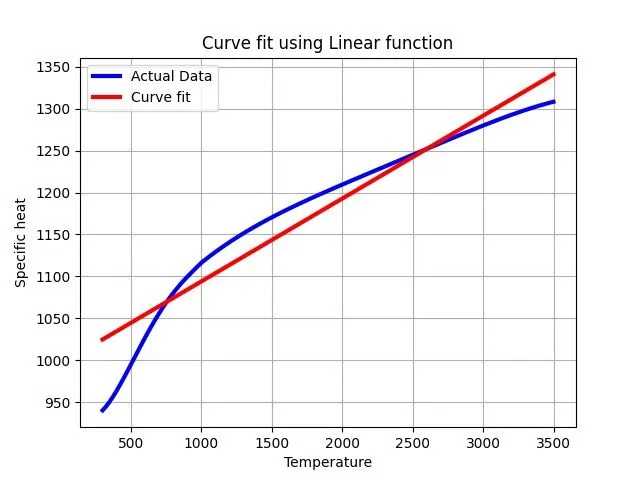
• A plot is created for the original function and the new function (created by curve fitting).

Python Code

# Linear function
import numpy as np 
import matplotlib.pyplot as plt 
from scipy.optimize import curve_fit

# Curve fit function
def func(t,a,b):
	return a*t+b 

# Reading thermodynamic data
def read_file():
	temperature=[]
	cp=[]
	for line in open('data','r'):
		values=line.split(',')
		temperature.append(float(values[0]))
		cp.append(float(values[1]))
	return temperature,cp
[temp,cp]=read_file()
popt,pcov= curve_fit(func,temp,cp)
fit_cp= func(np.array(temp),*popt)
# Error estimation

# mean CP calculation
totalcp=0
for i in range(0,len(cp)):
	totalcp=totalcp+cp[i]
meancp=totalcp/len(cp)
print(popt)

# SSE,SSR and SST estimation
# individual values
sse=[]
ssr=[]
for j in range(0,len(cp)):
	term1=fit_cp[j]-cp[j]
	sse.append(pow(term1,2))
	term2=fit_cp[j]-meancp
	ssr.append(pow(term2,2))
# summation of sse and ssr
SSE=0
SSR=0
for k in range(0,len(sse)):
	SSE=SSE+sse[k]
	SSR=SSR+ssr[k]
	
#SST calculation
SST=SSE+SSR
R=(SSR/SST)
print(R)


plt.plot(temp,cp,color='blue',linewidth=3)
plt.plot(temp,fit_cp,color='red',linewidth=3)
plt.legend(['Actual Data','Curve fit'])
plt.xlabel('Temperature')
plt.ylabel('Specific heat')
plt.show()

Output:

Cubic function:

Procedure

• numpy" library function is used to perform array operations in python.
• "mathplotlib" is used for plotting purposes.
• "scipy'' is used to import curve fit data.
• First a cubic function (a*t^3+b*t^2+c*t+d) is created using 'def' function.
• Then another function read file is created which reads and returns the temperature, specific heat values from the data.
• In the read file function, a for loop is created which reads specific heat and its corresponding temperature one by one. 'data' represents file name and 'r' represents the read option.
• In order to collect the data to perform operations, the function is called by using read_file().
• curve_fit command is used to perform curve fit operations.
• curve_fit takes function type, temperature, specific heat values from the data and returns optimized coefficient values(popt) and corresponding variance(pcov) for a new function that mimics the original function.
• Modified cp values are generated by using fit_cp which sends the optimized coefficient values(popt) and temperature from the data.
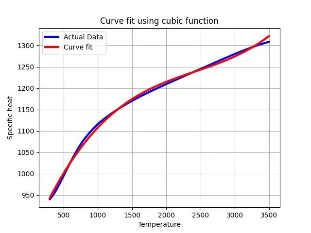
• A plot is created for the original function and the new function (created by curve fitting). Python Code

  # Cubic function
  import numpy as np 
  import matplotlib.pyplot as plt 
  from scipy.optimize import curve_fit
  
  # Curve fit function
  def func(t,a,b,c,d):
  	return a*pow(t,3)+b*pow(t,2)+c*t+d 
  
  # Reading thermodynamic data
  def read_file():
  	temperature=[]
  	cp=[]
  	for line in open('data','r'):
  		values=line.split(',')
  		temperature.append(float(values[0]))
  		cp.append(float(values[1]))
  	return temperature,cp
  [temp,cp]=read_file()
  popt,pcov= curve_fit(func,temp,cp)
  fit_cp= func(np.array(temp),*popt)
  # Error estimation
  
  # mean CP calculation
  totalcp=0
  for i in range(0,len(cp)):
  	totalcp=totalcp+cp[i]
  meancp=totalcp/len(cp)
  print(popt)
  
  # SSE,SSR and SST estimation
  # individual values
  sse=[]
  ssr=[]
  for j in range(0,len(cp)):
  	term1=fit_cp[j]-cp[j]
  	sse.append(pow(term1,2))
  	term2=fit_cp[j]-meancp
  	ssr.append(pow(term2,2))
  # summation of sse and ssr
  SSE=0
  SSR=0
  for k in range(0,len(sse)):
  	SSE=SSE+sse[k]
  	SSR=SSR+ssr[k]
  	
  #SST calculation
  SST=SSE+SSR
  R=(SSR/SST)
  print(R)
  
  
  plt.plot(temp,cp,color='blue',linewidth=3)
  plt.plot(temp,fit_cp,color='red',linewidth=3)
  plt.legend(['Actual Data','Curve fit'])
  plt.title('Curve fit using cubic function')
  plt.xlabel('Temperature')
  plt.ylabel('Specific heat')
  plt.grid()
  plt.show()
  ​

Conclusion:

From the above plots(linear and cubic) it can be concluded that the cubic curve matches exactly with the original curve and the residue are far fewer when compared to the linear curve.

What needs to be done in order to make the curve fit perfect?

To determine the perfect curve fit following methods needs to be followed

• Sum of squares due to Error
• R-squared
• Adjusted R-square
• Root meet square error

For this challenge, the R-square method is used

R-squared sometimes referred to as the coefficient of determination, is a measure of how well a linear regression model fits a dataset. It represents the proportion of the variance in the response variable that can be explained by the predictor variable.

The value for R-squared can range from 0 to 1. A value of 0 indicates that the response variable cannot be explained by the predictor variable at all. A value of 1 indicates that the response variable can be perfectly explained without error by the predictor variable.

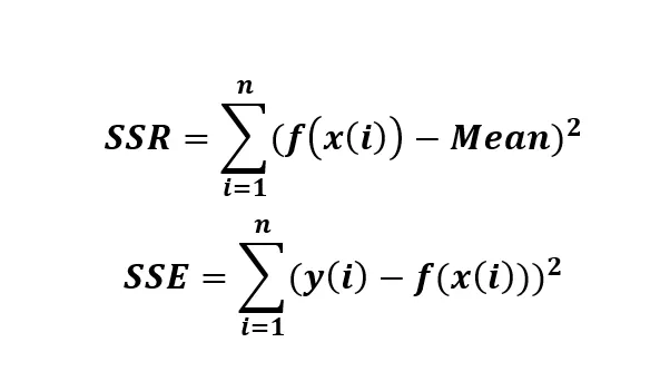
Using SSR and SST, we can calculate R-squared as:

R-squared = SSR / SST

SST(Sum of the squared total)=SSE(Sum of squared error)+SSR(Sum of the square of regression)

Show empirically as to how well your curve has been fit.

For cubic function

R-squared value is

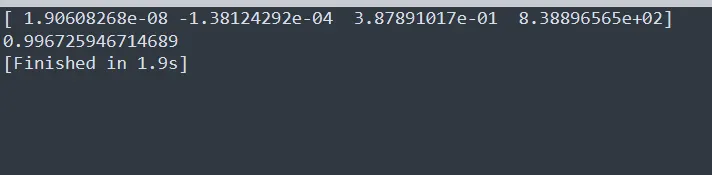
R-squared=0.996725946714689 Which is closer to 1

For Linear Function:

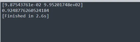
R-squared=0.9248776260524184

From the above values, it can be concluded that the cubic function has a better fit when compared to the linear function.