Curve fittting using Python

Curve fitting

Curve fitting is the process of constructing a curve, or mathematical functions, which posses the closest proximity to the real dataset. Curve fitting can construct a mathematical relation between the observed dataset and parameter values. It is highly effective in the mathematical modeling of some natural processes.

Curve fitting can involve either interpolation, where an exact fit to the data is required, or smoothing, in which a "smooth" function is constructed that approximately fits the data. A related topic is regression analysis, which focuses more on questions of statistical inference such as how much uncertainty is present in a curve that is fit to data observed with random errors.

Regression analysis is primarily used for two conceptually distinct purposes. First, regression analysis is widely used for prediction and forecasting, where its use has substantial overlap with the field of machine learning. Second, in some situations, regression analysis can be used to infer causal relationships between the independent and dependent variables. Importantly, regressions by themselves only reveal relationships between a dependent variable and a collection of independent variables in a fixed dataset.

Finding the degree of polynomial function to fit the dataset

Polynomial regression is a form of regression analysis in which the relationship between the independent variable x and the dependent variable y is modelled as an nth degree polynomial in x. Polynomial regression fits a nonlinear relationship between the value of x and the corresponding conditional mean of y.

The first degree polynomial equation

`y=ax+b`

is a line with slope '`a`'. A line will connect any two points, so a first degree polynomial equation is an exact fit through any two points with distinct x coordinates.

If the order of the equation is increased to a second degree polynomial, the following results:

`y=ax^{2}+bx+c`

This will exactly fit a simple curve to three points.

If the order of the equation is increased to a third degree polynomial, the following is obtained:

`y=ax^{3}+bx^{2}+cx+d`

This will exactly fit four points.

A more general statement would be to say it will exactly fit four constraints. Each constraint can be a point, angle, or curvature (which is the reciprocal of the radius of an osculating circle). Angle and curvature constraints are most often added to the ends of a curve, and in such cases are called end conditions.

Solving polynomial function and finding the goodness of fit

How to choose the best fit

Upon finding a curve that satisfies the data points there are 4 methods to measure the goodness of fit criteria.

The 4 methods are:-

1. The Sum of Square due to Error (SSE)

2. R-Square

3. Adjusted R-Square

4. Root Mean Square Error

1. The Sum of Square due to Error (SSE)

Let the function of the form `y=f(x)`

Assume the data points (x1,y1),(x2,y2),.....(xn,yn) are plotted as the values of function `y=f(x)`

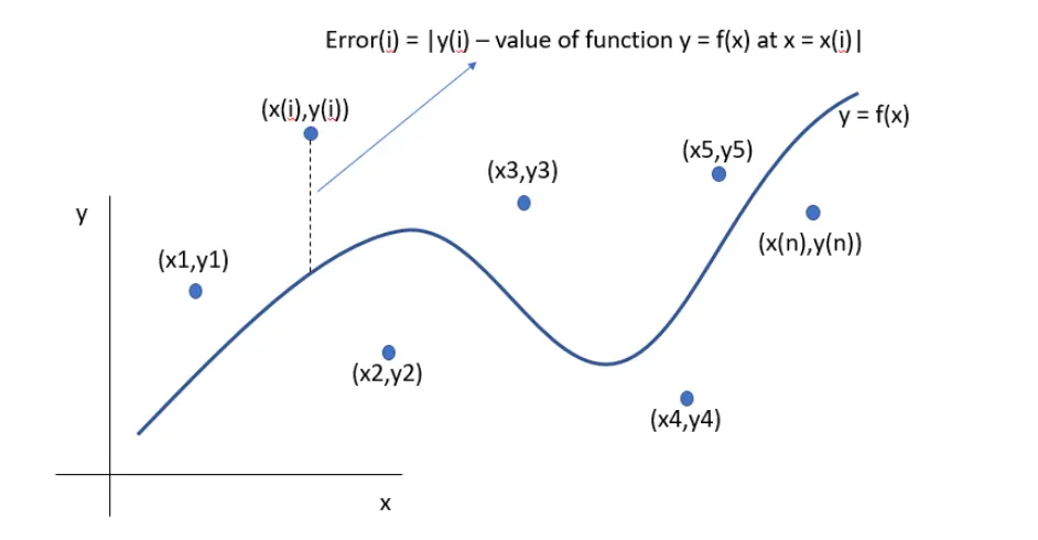
Suppose each of these points has an individual error (difference in y co-ordinate values) with the curve. The error at any general point 'i' can be given by the function,

`Er ro r(i)=|y_i-f(x_i)|`

where

`y_i` =value of y at i (corresponding value on curve at instant i)

`f(x_i)` = value of function `f(x)` at x=i

To remove the modulus sign, it is effective to take square of error.

The square of error of all the terms ranging from 1 to n is called Sum of Squared Error (`SSE`).

`SSE=sum_(i=1)^nEr ro r_i^2`

Assume the proposed equation is nth degree polynomial of the form,

`f(x)=A_1+A_2.x+A_3.x^2+...+A_n.x^(n-1)`

when we differentiate the (`SSE`) with each coefficient of the proposed equation `f(x)` respectively and equate to zero, we can find the minima and the value of coefficients of `f(x)`.

`Coefficient(f(x))[[(dS S E)/(dA_1)=0],[(d S S E)/(dA_1)=0],[.],[.],[.],[(dS S E)/(dA_n)=0]]`

2. R-Square

R-Square measures how successful the fit is in explaining the variation of the data. It is square of the correlation between the response value and the predicted response. It is also called the square of the multiple correlation coefficient and the coefficient of multiple determination.

It means that the higher the value of R-Square the better the fit, the lower it is the lousier the fit. The Value of R-Square ranges from 0 to 1.

0 for the worst possible fit and 1 for the best possible fit.

The value of R-Square can be calculated using the formula

``R^2=(SSR)/(SST)` where

SSR = is the sum of square of the difference between the values of the fitting function at a given point and the arithmetic mean of the data set.

SST= is the squared differences between the observed dependent variable and its mean. SST is Sum of Squares Total .

`SSR=sum_(i=1)^n (f(x_i)-mean)^2` and

`SSE=sum_(i=1)^n (f_i -f(x_i))^2`

`SST=SSR+SSE`

3. Adjusted R-Square

Adjusted R-Square is a normalizing variation of R-Square which neglects the variation of R-square due to insignificant independent variables.

Let

`y=f(x_1,x_2,x_3,...,x_n)` where `x_1,x_2,x_3,...,x_n` are the independent variables and `y` is the depedent variables.

If the value of `x_i` contributes to `y`, then `x_i` is a significant dependent variable and if the value of `x_i` does not contribute to `y`, then `x_i` is an insignificant dependent variable.

R_(adj)^2=1-[((1-R^2)(n-1))/(n-k-1)] where;

n=number of datapoints

k=number of independent variables

4. Root Mean Square Error (RMSE)

It is also known as the fit standard error and the standard error of the regression. It is an estimate of the standard deviation of the random component in the data. It is given by

`RMSE=sqrt((SSE)/(N))`

Curve Fit

scipy.optimize.curve_fit(f, xdata, ydata, p0=None, sigma=None, absolute_sigma=False, **kw)

Use non-linear least squares to fit a function, f, to data.

Assumes ydata = f(xdata, *params) + eps

Parameters:

f : callable The model function, f(x, ...). It must take the independent variable as the first argument and the parameters to fit as separate remaining arguments. xdata : An M-length sequence or an (k,M)-shaped array for functions with k predictors. The independent variable where the data is measured. ydata : M-length sequence The dependent data — nominally f(xdata, ...) p0 : None, scalar, or N-length sequence Initial guess for the parameters. If None, then the initial values will all be 1 (if the number of parameters for the function can be determined using introspection, otherwise a ValueError is raised). sigma : None or M-length sequence, optional If not None, these values are used as weights in the least-squares problem. absolute_sigma : bool, optional If False, sigma denotes relative weights of the data points. The returned covariance matrix pcov is based on estimated errors in the data, and is not affected by the overall magnitude of the values in sigma. Only the relative magnitudes of the sigma values matter. If True, sigma describes one standard deviation errors of the input data points. The estimated covariance in pcov is based on these values.

Returns:

popt : array Optimal values for the parameters so that the sum of the squared error of f(xdata, *popt) - ydata is minimized pcov : 2d array The estimated covariance of popt. The diagonals provide the variance of the parameter estimate. To compute one standard deviation errors on the parameters use perr = np.sqrt(np.diag(pcov)). How the sigma parameter affects the estimated covariance depends on absolute_sigma argument, as described above.

1. What does "popt" and "pcov" mean?

The curve fit returns the two arrays namely "popt" and "pcov" where popt gives the optimal values for the parameters so that the sum of the squared error of f(xdata, *popt) - ydata is minimized and pcov gives estimated covariance of popt. The diagonals provide the variance of the parameter estimate. To compute one standard deviation errors on the parameters use perr = np.sqrt(np.diag(pcov)).

2. What does np.array(temperature) do?

np.array(temperature) here is used to change the temperature list to an array. np.array is an array, any object exposing the array interface, an object whose __array__ method returns an array, or any (nested) sequence.

3. What does the * in *popt mean?

The * in *popt refers to optimal coeffcient and passes all the values of the fuction required for curve fit.

4. Write code to fit a linear and cubic polynomial for the Cp data. Explain if your results are good or bad?

Linear Polynomial Curve Fit

import numpy as np
import matplotlib.pyplot as plt
from scipy.optimize import curve_fit

# curve fit function
def func(t,a,b):
	return a*t+b

# reading thermodynamic data file
def read_file():
	temperature=[]
	cp=[]
	for line in open('data','r'):
		values=line.split(',')
		temperature.append(float(values[0]))
		cp.append(float(values[1]))
	return [temperature,cp]

# main program
temperature, cp=read_file()
popt, pcov=curve_fit(func, temperature, cp)
fit_cp=func(np.array(temperature), *popt)

plt.plot(temperature, cp,color='blue',linewidth=0.5)
plt.plot(temperature, fit_cp,color='red',linewidth=0.5)
plt.legend(['Actual Data', 'Curve Fit'])
plt.xlabel('Temperature [K]')
plt.ylabel('Cp')
plt.title('Linear Curve Fit')
plt.show()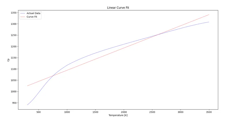

Cubic Polynomial Curve Fit

import numpy as np
import matplotlib.pyplot as plt
from scipy.optimize import curve_fit

# curve fit function
def func(t,a,b,c,d):
	return a*pow(t,3)+b*pow(t,2)+c*t+d

# reading thermodynamic data file
def read_file():
	temperature=[]
	cp=[]
	for line in open('data','r'):
		values=line.split(',')
		temperature.append(float(values[0]))
		cp.append(float(values[1]))
	return [temperature,cp]

# main program
temperature, cp=read_file()
popt, pcov=curve_fit(func, temperature, cp)
fit_cp=func(np.array(temperature), *popt)

plt.plot(temperature, cp,color='blue',linewidth=0.5)
plt.plot(temperature, fit_cp,color='red',linewidth=0.5)
plt.legend(['Actual Data', 'Curve Fit'])
plt.xlabel('Temperature [K]')
plt.ylabel('Cp')
plt.title('Cubic Curve Fit')
plt.show()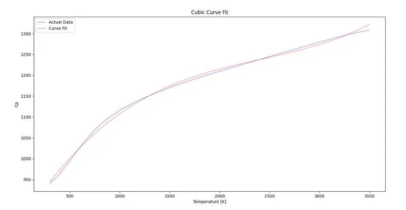

Comparison

It is seen that the cubic function gives a better reult for the given data as it resembles the original data better than the linear curve fit.

5. What needs to be done in order to make the curve fit perfect?

The curve fit can never be perfect. The main reason for that is the actual Experimental value and the ideal curve-fit value always vary. However, the value of actual data may come close to the ideal curve fit value. This can be seen by the code and graph shown. As the order of the equations increase, the value gets closer to the ideal value. There are other methods like dividing the data and curve fitting them separately or extrapolation.

6. Show empirically as to how well your curve has been fit?

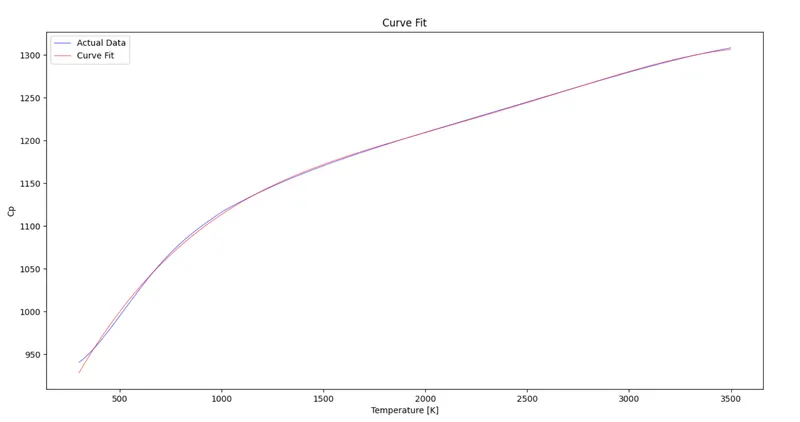
It is seen that by increasing the degree of the polynomial function the curve replicates the given data better.

import numpy as np
import matplotlib.pyplot as plt
from scipy.optimize import curve_fit

# curve fit function
def func(t,a,b,c,d,e):
	return a*pow(t,4)+b*pow(t,3)+c*pow(t,2)+d*t+e


# reading thermodynamic data file
def read_file():
	temperature=[]
	cp=[]
	for line in open('data','r'):
		values=line.split(',')
		temperature.append(float(values[0]))
		cp.append(float(values[1]))
	return [temperature,cp]

# main program
temperature, cp=read_file()
popt, pcov=curve_fit(func, temperature, cp)
fit_cp=func(np.array(temperature), *popt)

plt.plot(temperature, cp,color='blue',linewidth=0.5)
plt.plot(temperature, fit_cp,color='red',linewidth=0.5)
plt.legend(['Actual Data', 'Curve Fit'])
plt.xlabel('Temperature [K]')
plt.ylabel('Cp')
plt.title('Linear Curve Fit')
plt.show()