Week 5 - Curve fitting

Curve-Fitting Challenge

Aim:

1. Use python to write a code that fits data file provided for temperature and Cp.
2. Do a follow up research on Curve fitting process and answer some questions.

Problem Statement:

Data-science is a wide and new field in engineering and sciences. Data science gives us a vast set of data which needs to be studied for forecasting the future behavior of the data being studied. Thus, writing a program that can do the same with the set of data provided will be simplifying this process for the data scientists.

Theory:

Curve fitting is one of the most powerful and most widely used analysis tools in Origin. Curve fitting examines the relationship between one or more predictors (independent variables) and a response variable (dependent variable), with the goal of defining a "best fit" model of the relationship.

Assume data points (x1,y1),(x2,y2),(x3,y3),…..(x_n,y_n) and assume the best fit for these set of points will be y = f(x), the criterion under which the equation of the curve will be bet fit possible is as follows,

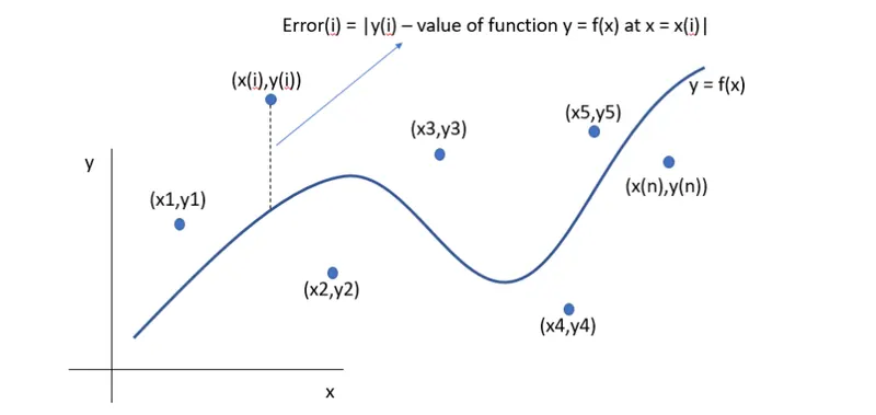
How to find the best fit curve?

One of best method is to use R-square method.

SSE(sum of squared errors) = ⁿΣ_(i=1) [Y(i) – f(x(i))]²

SSR(sum of squares of the regression) = ⁿΣ_(i=1) [f(x(i)) - mean]²

SST = SSE + SSR

R² = SSR/SST

Where;

R² = 1 implies perfect fit curve

0.95 < R² < 1 implies best fit curve

R² < 0.95 implies not good fit

Program:

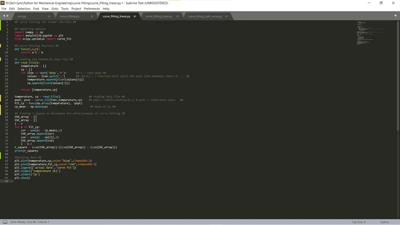
Linear function curve-fitting-

## curve fitting for linear function ##

## importing modules
import numpy as np
import matplotlib.pyplot as plt
from scipy.optimize import curve_fit

## curve fitting function ##
def func(t,a,b):
	return a*t + b

## reading the thermo-cp data file ##
def read_file():
	temperature = []
	cp = []
	for line in open('data','r'):      ## r = read mode ##
		values = line.split(',')       ## split(',') function will split the each line whenever there is ',' ##
		temperature.append(float(values[0]))
		cp.append(float(values[1]))

	return [temperature,cp]

temperature, cp = read_file()                  ## reading data file ##
popt, pcov = curve_fit(func,temperature,cp)    ## popt = coefficients(a,b,c) & pcov = covariance value   ##
fit_cp = func(np.array(temperature), *popt)
cp_mean = np.mean(cp)							## mean of Cp ##

## finding r_square to determine the effectiveness of curve-fitting ##
SSR_array = []
SSE_array = []
i = 0
for c in fit_cp:
	ssr = pow((c - cp_mean),2)
	SSR_array.append(ssr)
	sse = pow((c - cp[i]),2)
	SSE_array.append(sse)
	i = i+1
r_square = (sum(SSR_array))/((sum(SSR_array)) + (sum(SSE_array)))
print("r_square for linar curve fitting = ", r_square)

##ploting data ##
plt.plot(temperature,cp,color="blue",linewidth=3)
plt.plot(temperature,fit_cp,color="red",linewidth=3)
plt.legend(['actual data','curve fit'])
plt.xlabel('temperature [k]')
plt.ylabel('Cp')
plt.show()

Cubic function curve-fit-

## Cubic curve fitting ##

## importing modules ##
import numpy as np
import matplotlib.pyplot as plt
from scipy.optimize import curve_fit

## curve fitting function ##
def func(t,a,b,c,d):
	return a*(pow(t,3)) + b*(pow(t,2)) + c*t + d

## reading the thermo-cp data file ##
def read_file():
	temperature = []
	cp = []
	for line in open('data','r'):      ## r = read mode ##
		values = line.split(',')       ## split(',') function will split the each line whenever there is ',' ##
		temperature.append(float(values[0]))
		cp.append(float(values[1]))

	return [temperature,cp]

temperature, cp = read_file()					## reading data file ##
popt, pcov = curve_fit(func,temperature,cp)    ## popt = coefficients(a,b,c) & pcov =  covariance value   ##
fit_cp = func(np.array(temperature), *popt)
cp_mean = np.mean(cp)							## mean of Cp ##

## finding r_square to determine the effectiveness of curve-fitting ##
SSR_array = []
SSE_array = []
i = 0
for c in fit_cp:
	ssr = pow((c - cp_mean),2)
	SSR_array.append(ssr)
	sse = pow((c - cp[i]),2)
	SSE_array.append(sse)
	i = i+1
r_square = (sum(SSR_array))/((sum(SSR_array)) + (sum(SSE_array)))
print("r_square for Cubic curve fitting = ", r_square)

## plotting data ##
plt.plot(temperature,cp,color="blue",linewidth=3)
plt.plot(temperature,fit_cp,color="red",linewidth=3)
plt.legend(['actual data','curve fit'])
plt.xlabel('temperature [k]')
plt.ylabel('Cp')
plt.show()

Results:

linear program and result

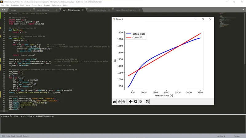
R² = 0.9248 ; which is less than 0.95 . therefore, linear curve fit is not accurate.

Cube program and result

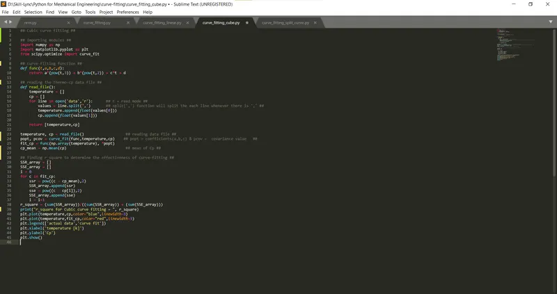
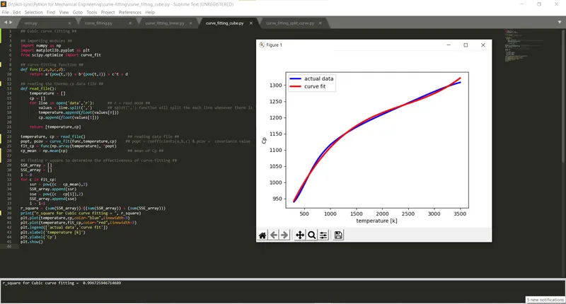
R² = 0.996 ; which is between 0.95 and 1 . therefore, cube curve fit is best fit for the data

Questions and answers:

1. What does popt and pcov mean?

Popt- gives optimum values for the coefficients in the function(a,b,c…etc.)

Pcov- The pcov variable contains the covariance matrix, which indicates the uncertainties and correlations between parameters. This is mostly useful when the data has uncertainties.

2. What does np.array(temperature) do?

Np.arrays creates an array from the data set provided within the paranthesis. In this case temperature is the dataset which is provided as a list.

3. What does the * in *popt mean?

The * notation will expand a list of values into the arguments of the function. This is useful if your function has more than one or two parameters.

4. Write code to fit a linear and cubic polynomial for the Cp data. Explain if your results are good or bad.

The code is provided in the program section and results are explained in results section

5. What needs to be done in order to make the curve fit perfect?

In order to make perfect fit, we must consider error estimates as well. Perfect fit means, the curve should fit the original curve without showing any errors (such as centring and scaling errors) in that particular degree of polynomial. Perfect fit can always be a best fit but best fit cannot be a perfect fit. Using cubic function can produce a greater but best fit for the curve. More perfect way to fit the curve is by splitting the curve into several parts to form the curve.

6. Show empirically as to how well your curve has been fit.

The graph in Results shows the curve fit for both linear and cubic curve fitting. Blue curve shows the data from read_file document. The red curve shows curve-fit. From the above two figures it is well clear that the cube function more accurately represent the data from read_file document on tempertures and specific heat data.

Also we can calculate R_square value for the two curve fits as;

1. R² = 0.9248 ; which is less than 0.95 . therefore, linear curve fit is not accurate.

2. R² = 0.996 ; which is between 0.95 and 1 . therefore, cube curve fit is best fit for the data

Discussion:

1. Program for linear and cubic curve fitting was done with python.
2. Accuracy of curve-fitting was determined from calculating R² The result shows that cube curve fitting shows more accurate fit towards the data.