Week 3 - Solving second order ODEs

PENDULUM CHALLENGE

Aim:

1. Write a program to solve the ODE that represent a pendulum with damping.
2. Also simulate the motion between 0-20 sec, for angular displacement=0, angular velocity=3rad/sec at time t=0.

Problem statement:

Ordinary differential equation has a vast application in the field of science and mathematics. One of those is in physics, to solve the problems related to pendulum. Damping makes these problems more difficult to solve with pen and paper. Thus coming up with a program to solve such equations are of great importance to the field of science.

Theory:

A pendulum is a body suspended from a fixed support so that it swings freely back and forth under the influence of gravity. When a pendulum is displaced sideways from its resting, equilibrium position, it is subject to a restoring force due to gravity that will accelerate it back toward the equilibrium position.We can generalise the equation representing pendulum with damping as following;

d²ᵠ/dt² + (b/m)*(dᵠ/dt) + (g/L)sinᵠ = 0

where;

ᵠ= angular displacement

b= damping coefficient

L= length of pendulum

m= mass of bob

g= acceleration due to gravity

t= time

Program:

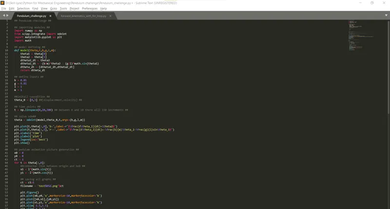
## Pendulum challenge ##

## importing modules ##
import numpy as np
from scipy.integrate import odeint
import matplotlib.pyplot as plt 
import math

## model defining ##
def model(theta,t,b,g,l,m):
	theta1 = theta[0]
	theta2 = theta[1]
	dtheta1_dt = theta2
	dtheta2_dt = -(b/m)*theta2 - (g/l)*math.sin(theta1)
	dtheta_dt = [dtheta1_dt,dtheta2_dt]
	return dtheta_dt

## define inputs ##
b = 0.05
g = 9.81
l = 1
m = 1

##initail coondition ##
theta_0 = [0,3] ##[displacement,velocity] ##

## time points ##
t = np.linspace(0,20,300) ## between 0 and 10 there will 150 increments ##

## solve ode##
theta = odeint(model,theta_0,t,args=(b,g,l,m))

plt.plot(t,theta[:,0],'b-',label=r'$\frac{d\theta_1}{dt}=\theta2$')
plt.plot(t,theta[:,1],'r--',label=r'$\frac{d\theta_2}{dt}=-\frac{b}{m}\theta_2-\frac{g}{l}sin\theta_1$')
plt.xlabel('time')
plt.ylabel('plot')
plt.legend(loc='best')
plt.show()

## pedulam animation picture generation ##
x0 = 0 
y0 = 0
ct = 1
for t in theta[:,0]:
	##connecter line between origin and bob ##
	x1 = l*(math.sin(t))
	y1 = -l*(math.cos(t))

	## saving all graphs ##
	ct = ct+1
	filename = 'test%05d.png'%ct
		
	plt.figure()
	plt.plot(x0,y0,'o',markersize=10,markerfacecolor='k')
	plt.plot([x0,x1],[y0,y1])
	plt.plot(x1,y1,'o',markersize=10,markerfacecolor='k')
	plt.xlim(-1.5,1.5)
	plt.ylim(-1.2,1)

	plt.savefig(filename)

Problems Faced:

The main problem faced during the challenge was to create animation from the angular displacements received from the function. The mentioned issue was discussed with the course guide and was resolved.

Results:

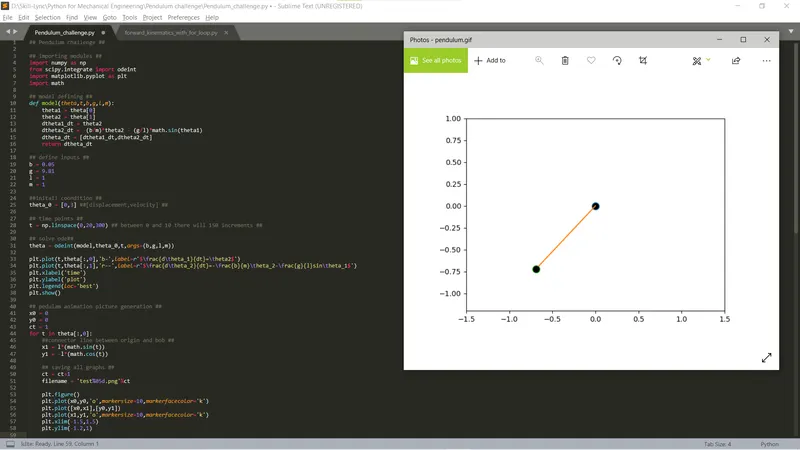
Output animation link: https://drive.google.com/file/d/1YY31ddI1xYsdmdbXwEtfujl-afxXOAcY/view?usp=sharing

Discussion:

1. ODE was solved using python for pendulum with damping.
2. Animation was created for the mentioned pendulum inputs.