Week 5 - Curve fitting
Objective:
To write a code for curve fitting using python and to answer the following questions.
1. What does popt and pcov mean?
2. What does np.array(temperature) do?
3. What does the * in *popt mean?
4. Write code to fit a linear and cubic polynomial for the Cp data. Explain if your results are good or bad.
5. What needs to be done in order to make the curve fit perfect?
6. Show empirically as to how well your curve has been fit.
Problem Statement:
- Curve fitting is the process of constructing a curve, or mathematical function, that has the best fit to a series of data points, possibly subject to constraints.
- It examines the relationship between one or more predictors (independent variables) and a response variable (dependent variable), with the goal of defining a "best fit" model of the relationship.
- In order to make perfect fit, we must consider error estimates as well. Perfect fit means, the curve should fit the original curve without showing any errors (such as centering and scaling erros) in that perticular degree of polynomial.
LINEAR POLYNOMIAL:
`ax+b=0`
CUBIC POLYNOMIAL:
`ax^3+bx^2+cx+d=0`
Solutions:
1. What does popt and pcov mean?
ANS:popt- An array of optimal values for the parameters which minimizes the sum of squares of residuals. pcov-2d array which contains the estimated covariance of popt. The diagonals provide the variance of the parameter estimate.
2. What does np.array(temperature) do?
ANS: it is an array to store values of different temperature. Basically, it saves all the values of temperature in an array from the sequence, so all the values can be called for each value of cp at every temperature.
3. What does the * in *popt mean?
ANS:generally this direct compilers reference to all the values(* means all) stored in popt array.
4. What needs to be done in order to make the curve fit perfect?
ANS:in order to make curve fit perfect we need to use split wise method in which we devide the given data in number of multiple parts
5.Show empirically as to how well your curve has been fit.
ANS:In order to make perfect fit, we must consider error estimates as well. Perfect fit means, the curve should fit the original curve without showing any errors (such as centering and scaling erros) in that perticular degree of polynomial.
Python code procedure:
- import required libraries for the smooth running of the programme
- define the curve fit function
- import the values of data temperature and cp divide them with ,
- create empty arrays of temperature and cp files
- append the float values
- return temperature and cp values
- use popt and pcov function 2d arrays
- plot the graphs of temperature and cp
- and plot graph between temperature and fit_cp
- use the same procedure for cubic polynomial equation
- now use the split wise method to split data into n number of parts
- use a, b as temperature ,cp
- use popt and pcov function to create arrays
- use plot command to plot the values on graphs
- save the graphs
- observe the graphs for error spotting
Python code:
import numpy as np
from scipy.optimize import curve_fit
import matplotlib.pyplot as plt
import math
#linear polynomial case 1
#curve fit function
def func(x,a,b):
	return a*x+b


# reading thermo dynamic data file
def read_file():
	temperature = []
	cp= []
	for line in open ('data','r'):
		values = line.split(',')
		temperature.append(float(values[0]))
		cp.append(float(values[1]))

	return [temperature,cp]

#main program
temperature,cp= read_file()
popt,pcov =curve_fit(func, temperature,cp)
fit_cp = func(np.array(temperature),*popt)

plt.plot(temperature,cp,'b-',linewidth=3,label=r'$data$')
plt.plot(temperature,fit_cp,'r-',linewidth=3,label=r'$ax+b$ (linear polynomial)curve_fit')
plt.title('general method')
plt.legend()#['actual data','curve fit']
plt.xlabel('temperature [k]')
plt.ylabel('cp')
plt.show()

#*********************************************************************************************************************
#cubic polynomial case 2
#curve fit function
def func(x,d,a,b,c):
	return a*x**3+b*x**2+c*x+d


# reading thermo dynamic data file
def read_file():
	temperature = []
	cp= []
	for line in open ('data','r'):
		values = line.split(',')
		temperature.append(float(values[0]))
		cp.append(float(values[1]))

	return [temperature,cp]

#main program
temperature,cp= read_file()
popt,pcov =curve_fit(func, temperature,cp)
fit_cp = func(np.array(temperature),*popt)

plt.plot(temperature,cp,'b-',linewidth=3,label=r'$data$')
plt.plot(temperature,fit_cp,'r-',linewidth=3,label=r'$ax^3+bx^2+cx+d$ (cubic polynomial)curve_fit')
plt.title('general method')
plt.legend()#['actual data','curve fit']
plt.xlabel('temperature [k]')
plt.ylabel('cp')
plt.show()

#*********************************************************************************************************************

#split vice method for linear method
def func(x,a,b):
	return a*x+b


# reading thermo dynamic data file
def read_file():
	temperature = []
	cp= []
	for line in open ('data','r'):
		values = line.split(',')
		temperature.append(float(values[0]))
		cp.append(float(values[1]))

	return [temperature,cp]

#main program
temperature,cp= read_file()
a= 0
b= 399
fit_cp =[]

for i in range(0,8):
	c=temperature[a:b+1]
	d = cp[a:b+1]

	popt, pcov = curve_fit(func, c,d)
	z = func(np.array(c), *popt)

	for j in z:
		fit_cp.append(j)

	a= b+1
	b= b+400

plt.plot(temperature,cp,'g-',linewidth=3,label=r'$data$')
plt.plot(temperature,fit_cp,'r-',linewidth=3,label=r'$ax+b$ (linear polynomial)curve_fit')
plt.title('split wice method')
plt.legend()#['actual data','curve fit']
plt.xlabel('temperature [k]')
plt.ylabel('cp')
plt.show()
#*********************************************************************************************************************
#split wice method for cubic polynomial
def func(x,a,b):
	return  a*x**3+b*x**2+c*x+d


# reading thermo dynamic data file
def read_file():
	temperature = []
	cp= []
	for line in open ('data','r'):
		values = line.split(',')
		temperature.append(float(values[0]))
		cp.append(float(values[1]))

	return [temperature,cp]

#main program
temperature,cp= read_file()
a= 0
b= 399
fit_cp =[]

for i in range(0,8):
	c=temperature[a:b+1]
	d = cp[a:b+1]

	popt, pcov = curve_fit(func, c,d)
	z = func(np.array(c), *popt)

	for j in z:
		fit_cp.append(j)

	a= b+1
	b= b+400

plt.plot(temperature,cp,'g-',linewidth=3,label=r'$data$')
plt.plot(temperature,fit_cp,'r-',linewidth=3,label=r'$ax^3+bx^2+cx+d$ (cubic polynomial)curve_fit')
plt.title('split wice method')
plt.legend()#['actual data','curve fit']
plt.xlabel('temperature [k]')
plt.ylabel('cp')
plt.show()
Results and Discussion:
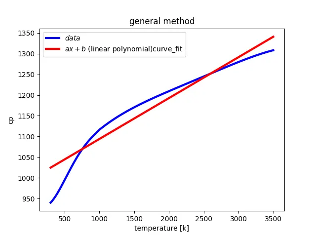
in the above graph we can see that we used linear equation for curve fit but it wasent that sucessfull and also the fit not at all matching the data graph and hence we found that the fit is not at all accurate.
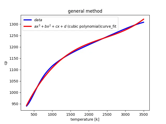
in order to make fit perfectly suite the data i found that cubic polynomial equation suits good enough to the data but not that accurate as we can see the both the lines clearly
and as there is error in the curve fit which needs to be rectified we use one among the number of error clearing methods which is split wice method.
in split wice method we split the given data into four different parts so that the curve plots four different times part wice along the actual data curve
the results of split wice method is given below
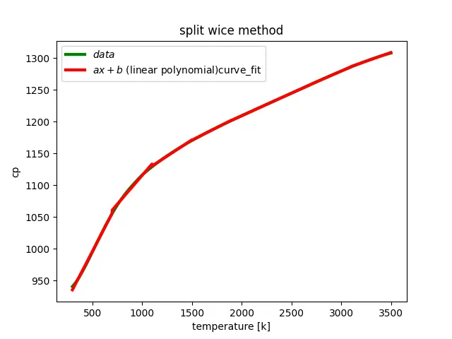
split wise method for linear polynomial
as we can observe that there is a huge difference in the graph for linear method itself from first general method to the split wise method
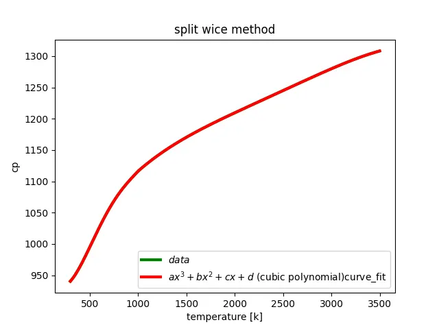
above graph is obtained from the cubic polynomial of the curve fit using split wice method as we cant even notice the actual data line because the curve fit is that accurate which got plotted most precisely on it and this i conclude the error spotting with the results of split wise method as it satisfys the requirements