Week 5 - Curve fitting
Aim:
To create a curve fitting for the given dataset and to find the best fit and perfect fit for that particular dataset using Python and Sublime text 3.
Objective
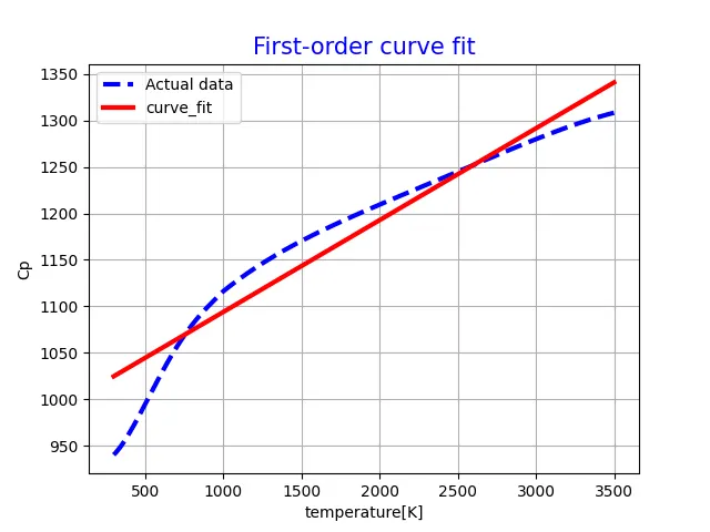
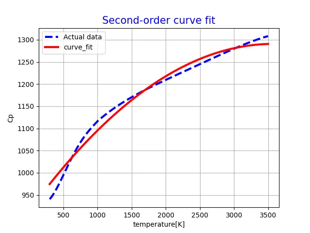
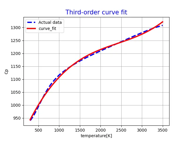
- To plot the linear and cubic fit curves along with the raw data points.
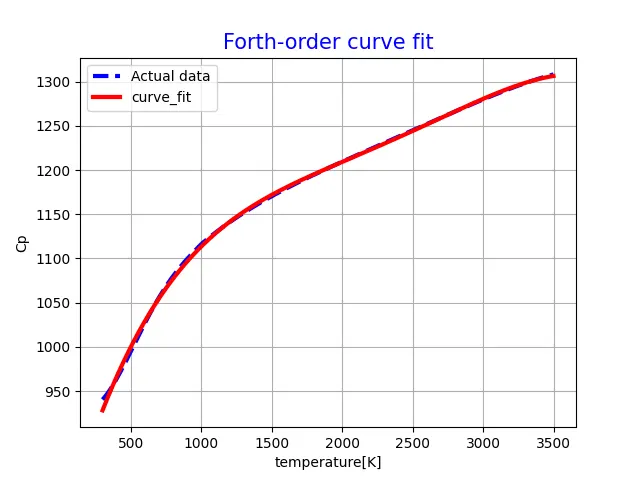
- To measure the fitness characteristics of the generated curves.
Theory:
Curve fitting is the way we represent a data spread by assigning the best fit function (curve) along with the range. Ideally, it will capture the trend in the data and allow us to make predictions of how the data series will behave in the future.
What needs to be done in order to make the curve fit perfect?
To make a curve fit perfect the error estimates should be considered. The perfect fit is a fit where it should match the original curve and shouldn't have any scaling and centring errors in that particular degree of the polynomial. The R^2 value must be equal to 1 and SSE=0.
What is the best fit?
A perfect fit can all the time be the best fit but the best fit may not be always a perfect fit. There are basically two methods to obtain the best fit.
- To increase the degree of the polynomial.
- To use the split-wise method i.e to split the data into folds and do the curve fitting for it.
Types Curve fitting :
(i)linear regression
it's when the data is fit to a straight line. Although there might be some curve to your data, a straight line provides a reasonable with enough fit to make forecasts.
Since the equation of a generic straight line is always given by f(x)= a x + b,
the question becomes: what a and b will give us the best fit line for our data
Considering the vertical distance from each point to a prospective line as an error, and summing them up over our range, gives us a concrete number that expresses how far from ‘best’ the prospective line is.
A line that provides a minimum error can be considered the best straight line.
Since it’s the distance from our points to the line we’re interested in—whether it is positive or negative distance is not relevant—we square the distance in our error calculations. This also allows us to weigh greater errors more heavily. So this method is called the least square approach.
(ii) Polynomial curve fitting
It's when we fit our data to the graph of a polynomial function. The same least-squares method can be used to find the polynomial, of a given degree, that has a minimum total error.
To choose the best fit for the curve the following four parameters help us to measure the goodness of fit criteria or how well the equations are representing the given data points:
- The sum of squares due to error,
- R-square
- Adjusted R-square,
- Root mean squared error
Equations used to fitness characteristic
- Error =|y(i)−f(x(i))|,
- SSE (sum of squared error) = `sum_(i=1)^N(error(i))^2`
- SSR (sum of the square of regression) = `sum_(i=1) ^N(f(x(i))−Mean)^2`
- SST (sum of the squared total) = SSE+SSR
- R^2 ( R squared) = SSR/SST
- RMSE (root mean squared error) = √(SSE/n)
where n is the total number of data points available.
The raw data of Temperature (K) and specific heat (kJ/kcalK) is obtained from here: Data
Python program
import numpy as np
import matplotlib.pyplot as plt
from scipy.optimize import curve_fit


t=input("let's create a curve that matches to given thermodynamic data")
#linear fit function
def func_1(t,a,b):
	return a*t+b

#curve fit function
def func_2(t,a,b,c):
	return a*pow(t,2)+b*t+c

#cubic curve fit function
def func_3(t,a,b,c,d):
	return a*pow(t,3)+b*pow(t,2)+c*t+d

#quadratic curve fit function
def func_4(t,a,b,c,d,e):
	return a*pow(t,4)+b*pow(t,3)+c*pow(t,2)+d*t+e

#reading thermodynamic data file
def read_file():
	temperature = []
	cp = []
	for line in open('data','r'):
		values = line.split(',')
		temperature.append(float(values[0]))
		cp.append(float(values[1]))
	return [temperature,cp]

# Main program
temperature,cp = read_file()
s = np.sum(cp)
l = np.size(cp)
m = s/l
print('\nMean of all cp :\n',m)
# For curve fit
linear_sse = 0
linear_ssr = 0
p = [1,2,3,4]
g = ['0','First' , 'Second', 'Third' ,'Forth']
for j in p:
	print('Generating ',g[j],'- order curve to fit given curve\n')
	if j == 1:
		popt, pcov = curve_fit(func_1,temperature,cp)
		fit_curve =func_1(np.array(temperature),*popt)
		for i in range(l):
		    linear_error = abs((np.sum((cp[i] - fit_curve[i]))))
		    linear_sse = linear_sse+pow(linear_error,2)
		    linear_ssr = linear_ssr+ np.sum(pow((fit_curve[i] - m),2))

	if j == 2:
		popt,pcov = curve_fit(func_2,temperature,cp)
		fit_curve =func_2(np.array(temperature),*popt)
		for i in range(l):
		    linear_error = abs((np.sum((cp[i] - fit_curve[i]))))
		    linear_sse = linear_sse+pow(linear_error,2)
		    linear_ssr = linear_ssr+ np.sum(pow((fit_curve[i] - m),2))

	if j == 3:
		popt,pcov = curve_fit(func_3,temperature,cp)
		fit_curve =func_3(np.array(temperature),*popt)
		for i in range(l):
		    linear_error = abs((np.sum((cp[i] - fit_curve[i]))))
		    linear_sse = linear_sse+pow(linear_error,2)
		    linear_ssr = linear_ssr+ np.sum(pow((fit_curve[i] - m),2))

	if j == 4:
		popt,pcov = curve_fit(func_4,temperature,cp)
		fit_curve =func_4(np.array(temperature),*popt)
		for i in range(l):
		    linear_error = abs((np.sum((cp[i] - fit_curve[i]))))
		    linear_sse = linear_sse+pow(linear_error,2)
		    linear_ssr = linear_ssr+ np.sum(pow((fit_curve[i] - m),2))

	#ploat section
	plt.plot(temperature,cp,'b--',linewidth =3)
	plt.plot(temperature,fit_curve,color = "red",linewidth =3)
	plt.legend(['Actual data','curve_fit'])
	plt.xlabel('temperature[K]')
	plt.ylabel('Cp')
	plt.grid()
	plt.title(g[j]+'-order curve fit',color='b',fontsize=15)
	plt.savefig(g[j]+'-order curve fit.png')
	plt.show()

	#fitness characteristics
	print('fitness characteristics for ',g[j],'- order curve fit')
	linear_sst = linear_sse + linear_ssr
	print('linear_sst :',linear_sst)
	linear_R2 = linear_ssr/linear_sst
	print('linear_R2 :',linear_R2)
	linear_rmse = pow((linear_sse/l),0.5)
	print('linear_RMSE :',linear_rmse)
Output data:
let's create a curve that matches to given thermodynamic data

Mean of all cp :
 1182.785685525818
Generating  First - order curve to fit given curve

fitness characteristics for  First - order curve fit
linear_sst : 28793673.249584787
linear_R2 : 0.9248776260524184
linear_RMSE : 25.999093068195325

Generating  Second - order curve to fit given curve

fitness characteristics for  Second - order curve fit
linear_sst : 57587346.50015386
linear_R2 : 0.9530598852639668
linear_RMSE : 29.064350221001654

Generating  Third - order curve to fit given curve

fitness characteristics for  Third - order curve fit
linear_sst : 86381019.75638323
linear_R2 : 0.9676152390829476
linear_RMSE : 29.566813493878062

Generating  Forth - order curve to fit given curve

fitness characteristics for  Forth - order curve fit
linear_sst : 115174693.00888032
linear_R2 : 0.9756153120618613
linear_RMSE : 29.62525816022789

>>> 
Based on the above work, we can answer the following questions:
What do popt and pcov mean?
'popt' represents the matrix that stores and extracts the coefficients for the fitting functions according to the general equations defined.
popt : array, Optimal values for the parameters so that the sum of the squared residuals f(xdata, *popt) - ydata is minimized
'pcov' represents the square matrix that stores the estimated values of covariance of the coefficients above. The diagonal elements of this square matrix also represent a variance of that coefficients.
pcov : 2d array
The estimated covariance of popt. The diagonals provide the variance of the parameter estimate. To compute one standard deviation errors on the parameters used perr = np.sqrt(np.diag(pcov)).How the sigma parameter affects the estimated covariance depends on the absolute_sigma argument, as if True, sigma is used in an absolute sense and the estimated parameter covariance pcov reflects these absolute values. If False, only the relative magnitudes of the sigma values matter. The returned parameter covariance matrix pcov is based on scaling sigma by a constant factor.
What does np.array(temperature) do?
This command converts each value of the temperature data file into an array using numpy Library.
What does the * in *popt mean?
'*' , '*popt' indicates and returns each coefficient stored in popt array.