Week 5.2 - Literature review: ODE Stability

Aim: The aim of this study is to understand the stability of the ordinary differential equation (ODE) and its effect on the engineering solutions.

Introduction: Theoretically we assume (fuel + air = products of combustion). But in the real world scenarios, no reaction takes place in a single step. There are different elementary and intermediate reactions that reactants go through to form the final products. This entire set of reactions is called as ‘reaction mechanism’. For a solver to solve these reactions accurately, reaction rates are needed to be provided. These reaction rates are in the form of ODE. But as the different parameters of the ODE change, the ODE becomes unstable and tends to give inaccurate solutions. Hence, this study focuses on the stability of the ODE.

Coding Approach:

• ‘Math’ and ‘matplotlib.pyplot’ modules are imported in the python.
• A function named ‘explicit_euler’ is defined. It has parameters total time and ‘dt’. A time variable ‘t’ is created. It’s value ranges from 0 to total time with increment of ‘dt’. A matrix of zeros, ‘y’ is created that has same length as ‘t’. A ‘for’ loop is created in the same function. It iterates from 1 to the length of ‘t’. With each iteration, value of ‘y’ is changed as [y = y_old + dt*(1000*y_old – e^(-t_old). This function returns the value of ‘t’ and ‘y’.
• Similarly, a new function is created with the update rule of y as [y = (y_old – e^(-t_old)*dt)/(1+100*dt).
• Again, a similar function named analytical is created to compute the analytical value of the ODE. Its name is ‘analytical’ with the update rule of ‘y’ as [y = (e^(-100*t)*(1-e^(99t))/99].
• Then, values of ‘t’ and ‘y’ are plotted for all of the three functions using ‘matplotlip.pyplot’ module.

Code:

import numpy as np

import matplotlib.pyplot as plt

def explicit_euler(total_t,dt):

t = np.arange(0,total_t,dt)

y = np.zeros(len(t))

for i in range(1, len(t)):

y[i] = y[i-1] + dt*(-100*y[i-1] - np.exp(-t[i-1]))

return [t,y]

def implicit_euler(total_t,dt):

t = np.arange(0,total_t,dt)

y = np.zeros(len(t))

for i in range(1, len(t)):

y[i] = (y[i-1] - np.exp(-t[i-1])*dt)/(1+100*dt)

return [t,y]

def analytical(total_t,dt):

t = np.arange(0,total_t,dt)

y = np.zeros(len(t))

for i in range(1, len(t)):

y[i] = np.exp(-100*t[i])*(1-np.exp(99*t[i]))/99

return [t,y]

total_t = 0.1

dt = 1e-3

t, y_explicit = explicit_euler(total_t,dt)

t, y_implicit = implicit_euler(total_t,dt)

t, y_analytical = analytical(total_t,dt)

plt.plot(t, y_explicit, color = 'blue')

plt.plot(t, y_implicit, color = 'black')

plt.plot(t, y_analytical, color = 'orange')

plt.legend(['Explicit','Implicit', 'Analytical'])

plt.title('Parameter = 100, dt = 1e-3')

plt.show()

Results:

The original ordinary differential equation is: [dy/dt = -1000*y – e^(-t)].

Here the parameter multiplying ‘y’ is 1000 and ‘dt’ can be varied.

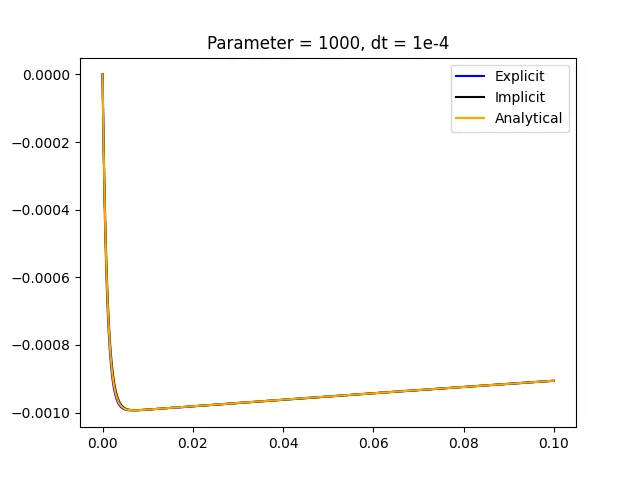
Figure (1): Results of explicit, implicit and analytical method when parameter is 1000 and dt = 1e-4.

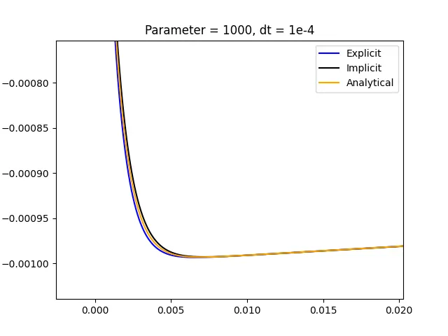
Figure (2): Results of explicit, implicit and analytical method when parameter is 1000 and dt = 1e-4.

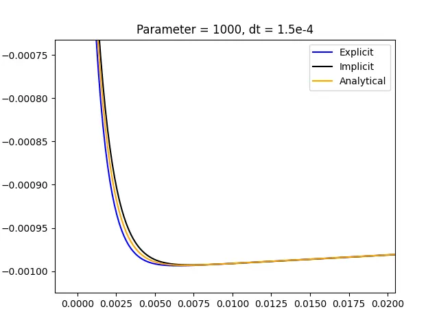
Figure (3): Results of explicit, implicit and analytical method when parameter is 1000 and dt = 1.5e-4.

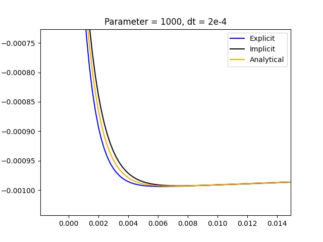
Figure (4): Results of explicit, implicit and analytical method when parameter is 1000 and dt = 2e-4.

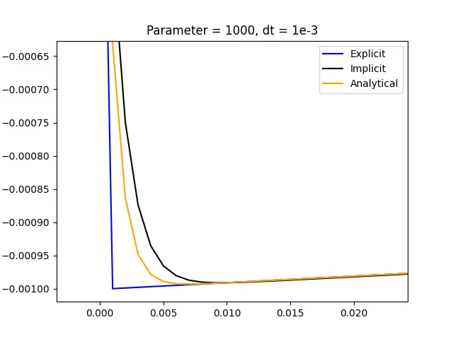
Figure (5): Results of explicit, implicit and analytical method when parameter is 1000 and dt = 1e-3.

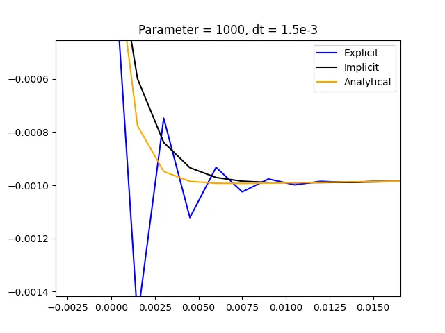
Figure (6): Results of explicit, implicit and analytical method when parameter is 1000 and dt = 1.5e-3.

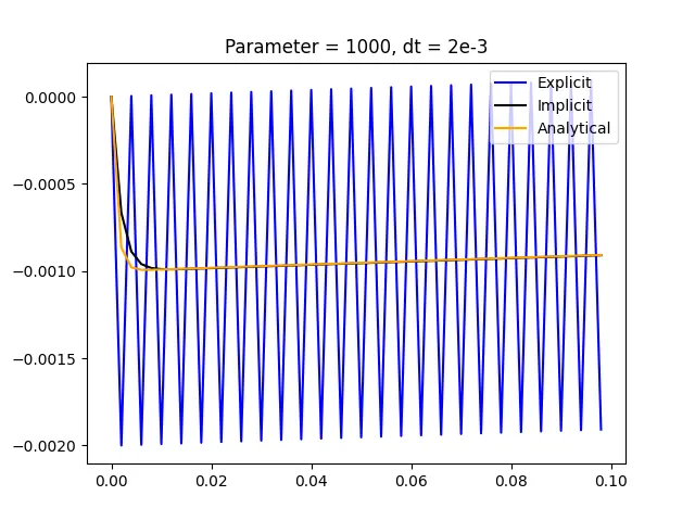
Figure (7): Results of explicit, implicit and analytical method when parameter is 1000 and dt = 2e-3.

As it can be seen from figures 1 to 7, as the ‘dt’ increases, the distortion starts increasing and when the ‘dt’ is 1e-3, the explicit solution starts deviating from the analytical and implicit solutions to a large extent. Implicit solution closely matches to the analytical solution until the ‘dt’ is in the order of e-4.

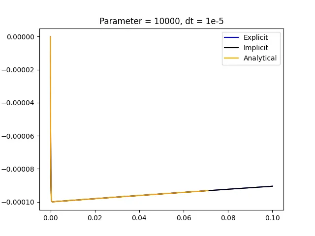
Figure (8): Results of explicit, implicit and analytical method when parameter is 10000 and dt = 1e-5.

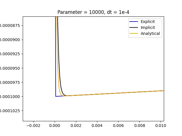
Figure (9): Results of explicit, implicit and analytical method when parameter is 10000 and dt = 1e-4.

To further perform the analysis, the parameter multiplying ‘y’ is changed to 10000. From the figure 8, it can be concluded that, the explicit, implicit and the analytical solutions match to a certain extent. But as the ‘dt’ is changed to 1e-4, as in figure 9, the explicit and the implicit solutions start deviating from the analytical solution.

From all the 9 results, it can be concluded that, the ODE remains stable until, if ‘y’ has the parameter multiplying it as (10)^i and ‘dt’ remains in the power of e-(i+1).

Answer for Question (2):

As the ODE becomes unstable, the solution starts deviating from the actual answer. Hence, it adversely affects the solution of the problem. This can lead to faulty design or unexpected data points.

Answer for Question (3):

Although for this problem stability condition was easy to derive, but for many real world problem involving complex functions and variables, it becomes difficult to derive the stability condition.