Week 5.1 - Non-Conformal Meshing and Solving a Cold plate model
In this challenge, 2 heated plates are getting cooled by water circulating inside the cold plate cavity and also by air externally by natural convection.
Problem Information:
|
Cabinet |
0.4 m x 0.3 m x 0.2 m |
||
|
Cabinet Openings |
Min X & Max X |
||
|
Solid Block |
Start Point (0.05,0.08,0.07) & dimensions of 0.3 m x 0.14m x 0.06m |
Block type :Solid |
Material : Al-Extruded |
|
Fluid Block |
Start Point (0.06,0.09,0.08) & dimensions of 0.28 m x 0.12m x 0.04m |
Block type :Fluid |
Material : Water (280 K) |
|
Inlet Pipe (Solid) |
(0.1,0,0.1) - Centre Point, height = 0.09 m and a = 0.015 m |
Block type :Solid |
Material : Al-Extruded |
|
Inlet Pipe (Fluid) |
(0.1,0,0.1) Centre Point, height = 0.09 m, radius = 0.01 m |
Block type :Fluid |
Material : Water (280 K) |
|
Outlet Pipe (Solid) |
(0.3,0,0.1) Centre Point, height = 0.09 m and a = 0.015 m |
Block type :Solid |
Material : Al-Extruded |
|
Outlet Pipe (Fluid) |
(0.3,0,0.1) Centre Point height = 0.09 m, radius = 0.01 m |
Block type :Fluid |
Material : Water (280 K) |
|
Heated Plate 1 |
located at (0.07,0.1,0.06) having dimensions of (0.260 m X 0.1m) in Z plane |
conducting thick 10mm |
200 W |
|
Heated Plate 2 |
located at (0.07,0.1,0.13) having dimensions of(0.260 m X 0.1m) in Z plane |
conducting thick 10mm |
200 W |
Inlet Pipe Opening
(0.1,0,0.1) Centre Point, radius = 0.01 m
Type: Opening
Geometry: Circular
Plane: X-Z
Y Velocity = 0.2 m/s
Outlet Pipe Opening
(0.3,0,0.1) Centre Point,radius = 0.01 m
Type: Opening
Geometry: Circular
Plane: X-Z
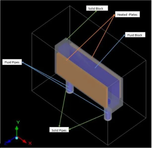
Geometry Information
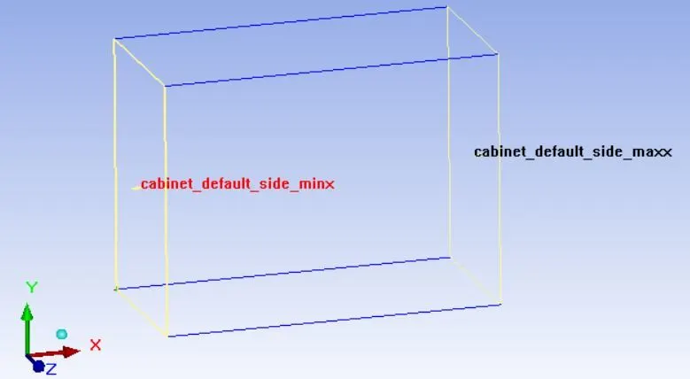
Cabinet Geometry
Shape : Prism
Location:
Specified by -> Start/end
Min X = 0
Max X = 400 mm
Min Y = 0
Max Y = 300 mm
Min Z = 0
Max Z = 200 mm
Properties :
Min X -> Opening
Max X -> Opening
Min Y -> Default
Max Y -> Default
Min Z -> Default
Max Z -> Default
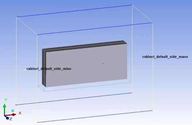
Fluid Block
Shape : Prism
Location:
Specified by -> Start/end
Min X = 60 mm
Max X = 340 mm
Min Y = 90 mm
Max Y = 210 mm
Min Z = 80
Max Z = 120 mm
Properties :
Block type : Fluid
Fluid material : water (@280 K)
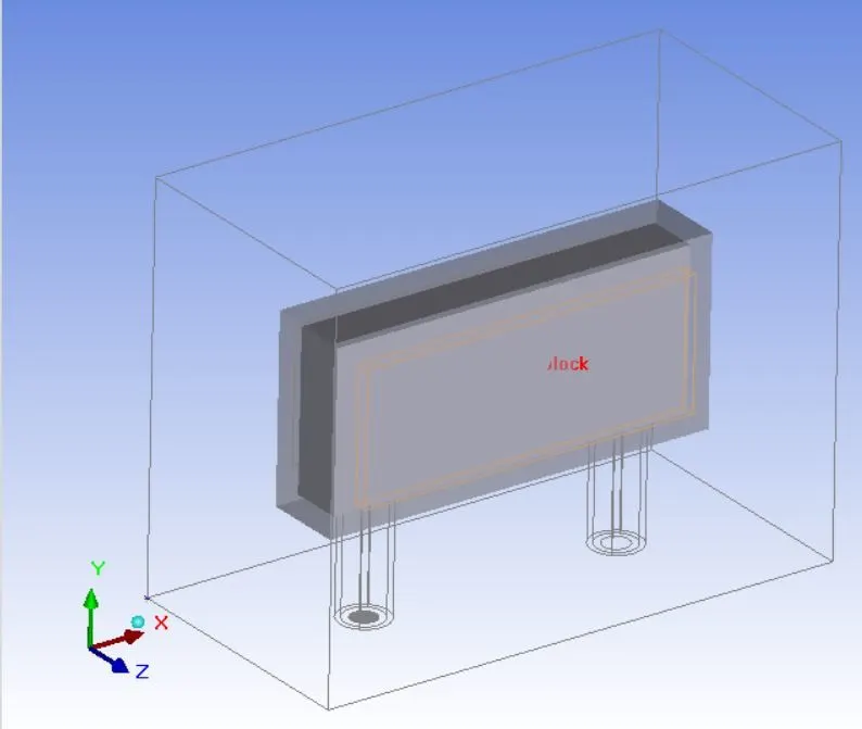
Solid Block
Shape : Prism
Location:
Specified by -> Start/end
Min X = 50 mm
Max X = 350 mm
Min Y = 80 mm
Max Y = 220 mm
Min Z = 70
Max Z = 130 mm
Properties :
Block type : solid
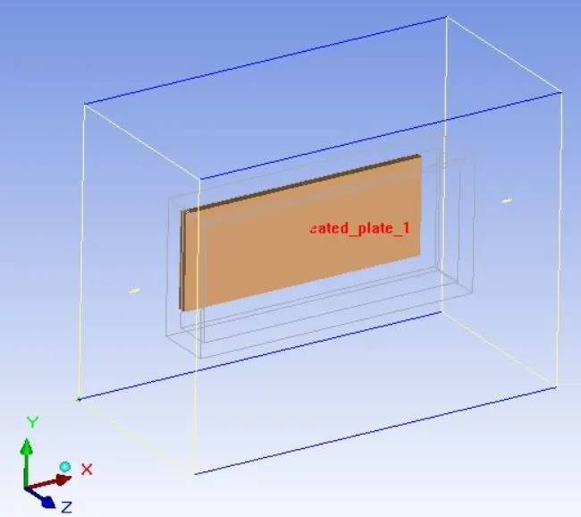
Hot Plate-1
Shape : Rectangle
Plane: X-Y
Location:
Specified by -> Start/end
Min X = 70 mm
Max X = 330 mm
Min Y = 100 mm
Max Y = 200 mm
Min Z = 60
Properties
Block type : solid
Thermal model : Conducting thick
Thermal Specification:
Thickness : 10 mm
Total Power : 200 W ; Constant
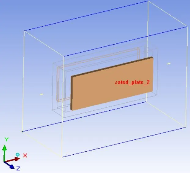
Hot Plate-2
Shape : Rectangle
Plane: X-Y
Location:
Specified by -> Start/end
Min X = 70 mm
Max X = 330 mm
Min Y = 100 mm
Max Y = 200 mm
Min Z = 130 mm
Properties
Block type : solid
Thermal model : Conducting thick
Thermal Specification:
Thickness : 10 mm
Total Power : 200 W ; Constant
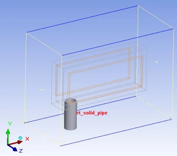
Inlet Solid Pipe
Shape: Cylinder
Plane : X-Z
Location:
Min X = 100 mm
Max Y = 0 mm
Min Z = 100 mm
Height = 90 mm
Radius = 19 mm
Internal Radius = 15 mm
Properties
Block type : solid
Thermal Specification:
Al-Extruded
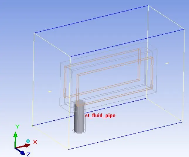
Inlet Fluid Pipe
Shape: Cylinder
Plane : X-Z
Location:
Min X = 100 mm
Max Y = 0 mm
Min Z = 100 mm
Height = 90 mm
Radius = 15 mm
Internal Radius = 0 mm
Properties
Block type : Fluid
Thermal Specification:
Water (@280 K)
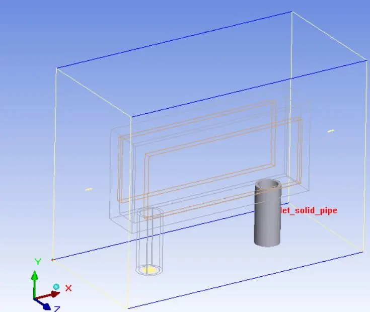
Outlet Solid Pipe
Shape: Cylinder
Plane : X-Z
Location:
Min X = 300 mm
Max Y = 0 mm
Min Z = 100 mm
Height = 90 mm
Radius = 19 mm
Internal Radius = 15 mm
Properties
Block type : solid
Thermal Specification:
Al-Extruded
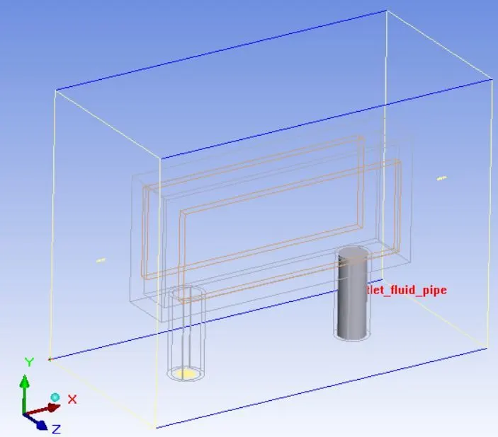
Outlet Fluid Pipe
Shape: Cylinder
Plane : X-Z
Location:
Min X = 300 mm
Max Y = 0 mm
Min Z = 100 mm
Height = 90 mm
Radius = 15 mm
Internal Radius = 0 mm
Properties
Block type : Fluid
Thermal Specification:
Water (@280 K)
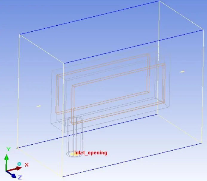
Inlet Opening
Type : Free
Shape : Circular
Plane : X-Z
Location
Center :
X = 100 mm
Y = 0 mm
Z = 100 mm
Radius = 10 mm
Temperature = ambient
Y Velocity = 0.2 m/s
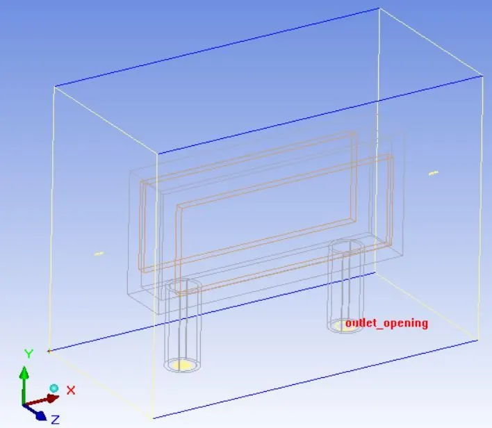
Outlet Opening
Type : Free
Shape : Circular
Plane : X-Z
Location
Center :
X = 300 mm
Y = 0 mm
Z = 100 mm
Radius = 10 mm
Temperature = ambient
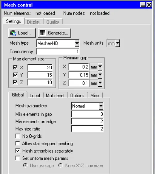
Meshing
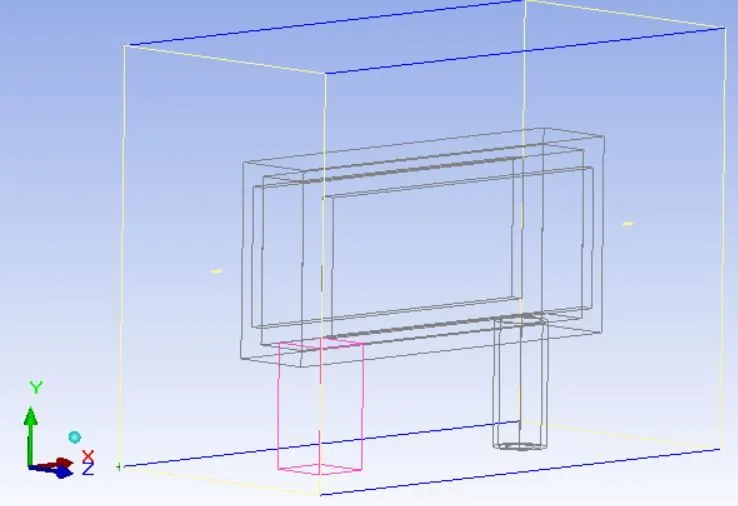
Create Assembly of inlet_Solid, Inlet_Fluid and inlet_Opening parts
Assembly-1
Defination : Internal assembly
Meshing : Meshing Separately
Slack setting
Min X = 2 mm
Max X = 2 mm
Min Y = 0 mm
Max Y = 0 mm
Min Z = 2 mm
Max Z = 2 mm
Mesh type : Default
Max element size
X = 2 mm
Y = 5 mm
Z = 2 mm
Minimum Gap
X = 0.02 mm
Y = 0.05 mm
Z = 0.02 mm
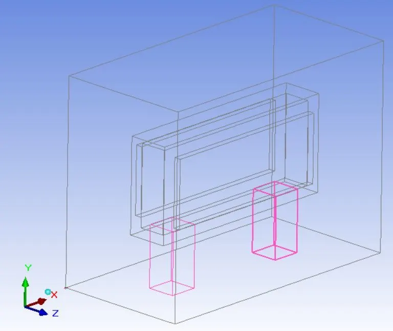
Create Assembly of outlet_Solid, Outlet_Fluid and Outlet_Opening parts
Assembly-2
Defination : Internal assembly
Meshing : Meshing Separately
Slack setting
Min X = 2 mm
Max X = 2 mm
Min Y = 0 mm
Max Y = 0 mm
Min Z = 2 mm
Max Z = 2 mm
Mesh type : Default
Max element size
X = 2 mm
Y = 5 mm
Z = 2 mm
Minimum Gap
X = 0.02 mm
Y = 0.05 mm
Z = 0.02 mm
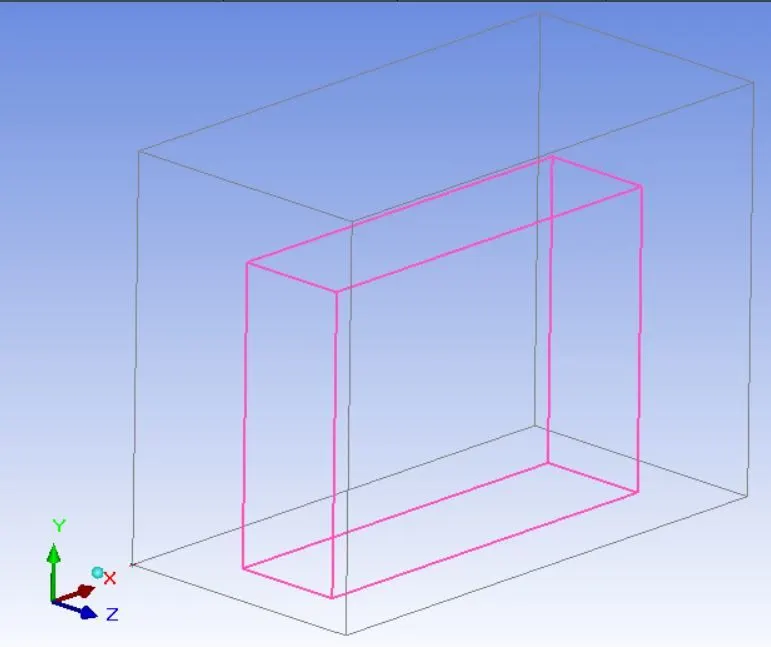
Create Assembly of Assembly-1, Assembly-2, Plate-1,Plate-2, Fluid_block,Solid_block
Assembly-3
Defination : Internal assembly
Meshing : Meshing Separately
Slack setting
Min X = 2 mm
Max X = 2 mm
Min Y = 0 mm
Max Y = 2 mm
Min Z = 2 mm
Max Z = 2 mm
Mesh type : Default
Max element size
X = 10.0 mm
Y = 7.5 mm
Z = 5.0 mm
Minimum Gap
X = 0.01 mm
Y = 0.075 mm
Z = 0.05 mm
Automatic case Check Tool
Macros -> Productivity -> Validation
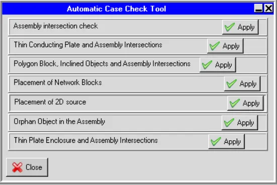
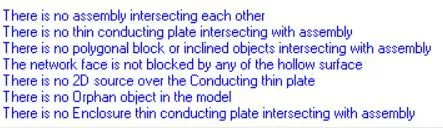
This check ensure geometry modelling is ok.
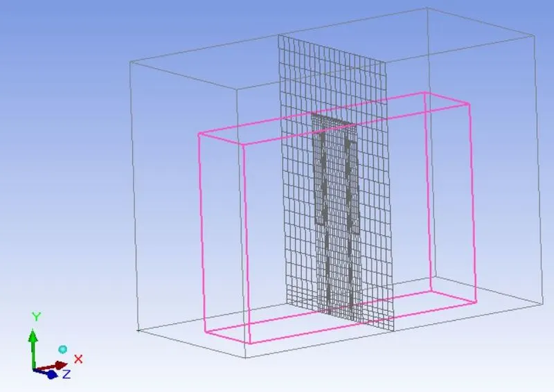
X-Plane
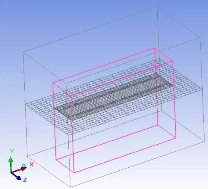
Y-Plane
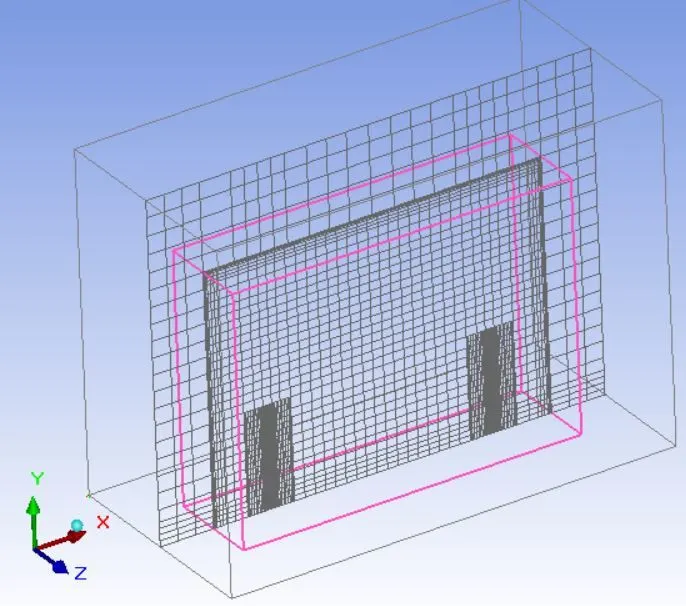
Z-plane
Quality
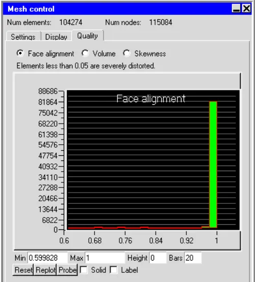
Face alignment : It is a measure of the relative alignment between two adjacent elements in the mesh. Above image shows the Face alignment histogram for different elements in the current mesh.
The value of face alignment ranges from 0 to 1.
Value greater than 0.1 is preffered and greater than 0.15 is better.
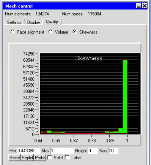
Skewness : It is a measure of how close to the ideal (equilateral/equiangular) a mesh element is. Above image shows the skewness histogram for different elements in the current mesh.
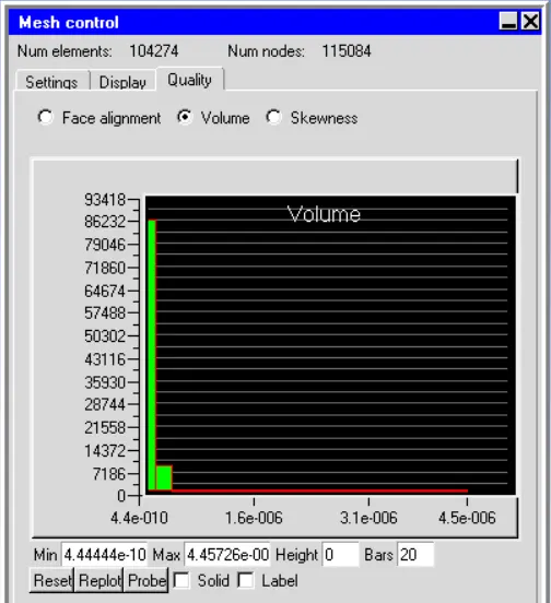
Volume :
Preferable Volume mesh should be 1E-12 for single precision and 1E-15 for double precision.
Solver
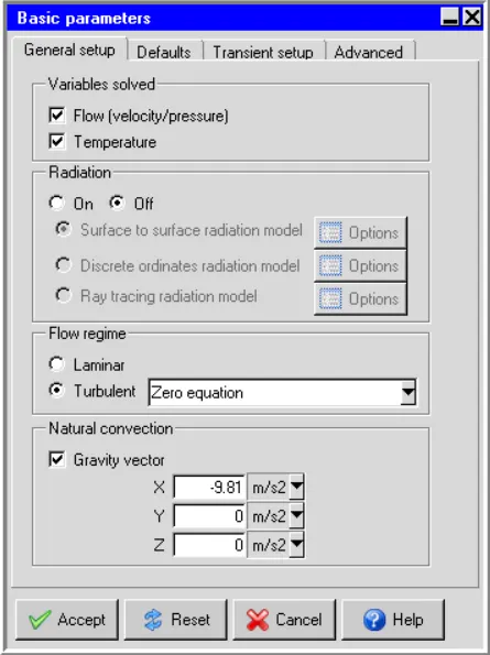
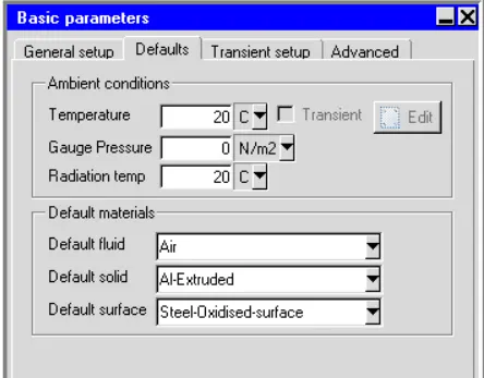
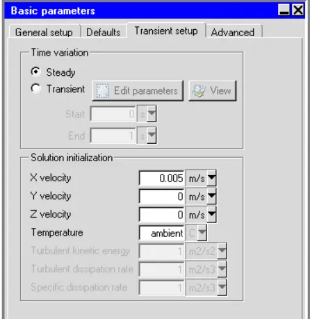
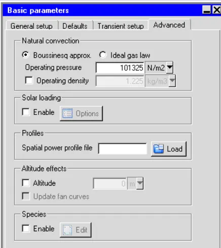
ANSYS Icepak package employs the FLUENT solver engine to solve the discretized governing equations within the computational domain. The following settings are applied in the Problem Setup and Solution settings nodes of the Model manager window
Solution Settings :
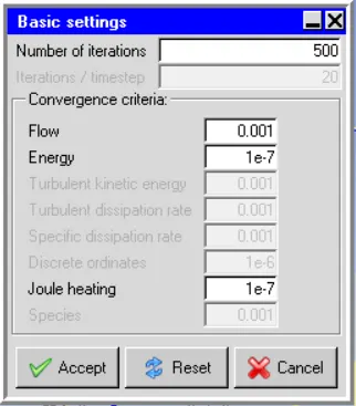
Basic Setting :
The image attached below shows the various parameters specified in the Basic settings node available within the solution settings node in the model manager window.

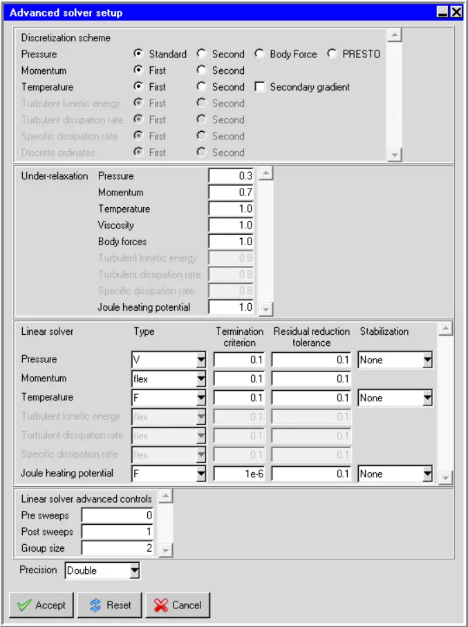
Advanced settings
The image attached below shows the various parameters specified in the Advanced settings node available within the solution settings node in the Model manager window.
Results :
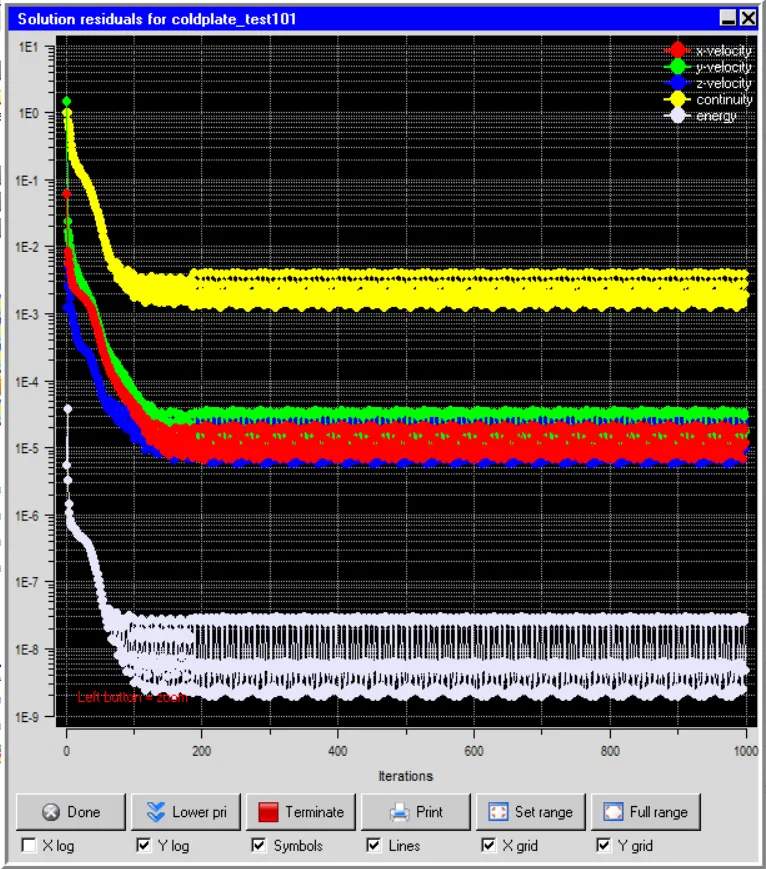
Residuals
The residuals for the following governing equations are monitored:
Temperature monitor plots
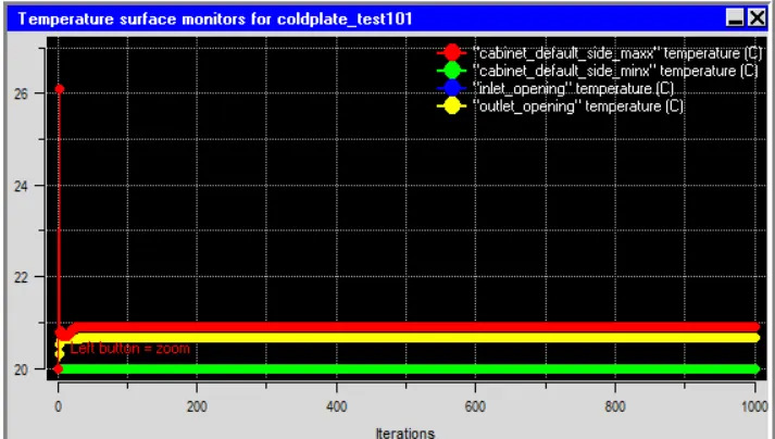
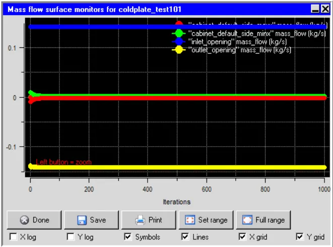
From above plot it is evident that from monitor surface average plots that water temperature has increased approximately by 1.0 degree C (from 20 degree C to 21.0 degree C)
Temperature Contours
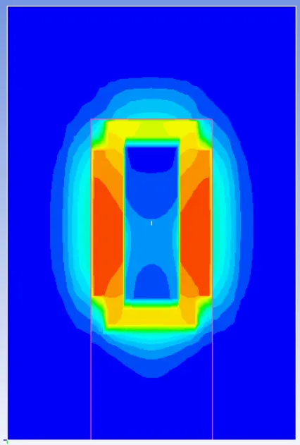
Temperature contours are plotted along different cut-planes as well as object faces to observe the temperature distribution throughout the domain at steady state.
Temperature contours plotted on the Z-Plane through the center
The image attached below shows the steady state temperature contours plotted on the cut-plane passing through the center of the cabinet and perpendicular to the Z-axis.
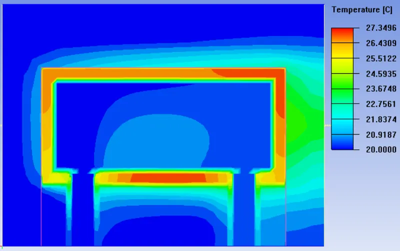
The plot clearly shows that water enters into cold plate cavity at ambient temperature (20 degree C) and as it moves further inside the cavity its temperature increases.This is because of the heat transfer from Solid_block to water.
Temperature contours plotted on the Y-Plane through the center
The image attached below shows the steady state temperature contours plotted on the cut-plane passing through the center of the cabinet and perpendicular to the Y-axis.
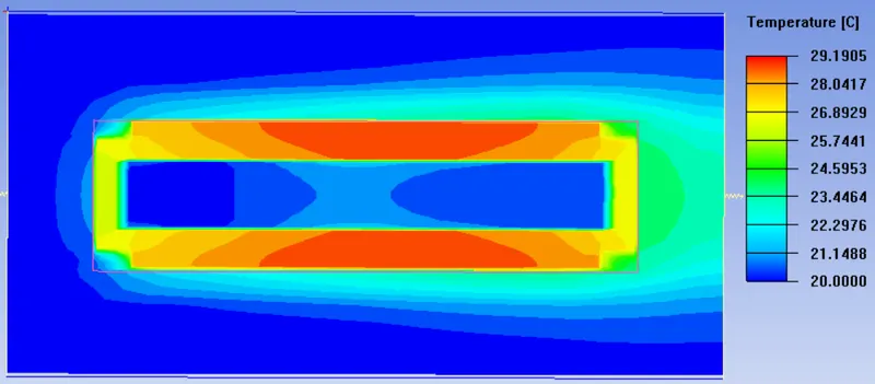
The plot shows that the heated plates achieve the highest temperature and as we move from the heated plates to Solid_block the temperature dereases. This indiacates that temperature gradient exists between heated plates and solid_block.
It is observed that temperature gradient is also present between solid_block and fluid_block.This indiacates that heat is lost from solid_block to fluid_block region.
To summarize, heat generated in heated plates is transferred to solid_block(by conduction) and further to fluid_block (by free convection). One more path of heat loss is between solid_block and water (by forced convection).
The contours also clearly show the presence of thermal boundary layers on the outer surfaces of the heated plates. These thermal boundary layers are formed as a result of heat transfer between the heated plates and ambient air ( by natural convection) and thermal boundary layer grows against the gravitational field.
Temperature contours plotted on the Z-Plane through the center
Fluid face temperature contours :
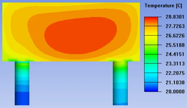
The image attached above shows the steady state temperature contours plotted on the outer faces of all the objects in the geometry that are defined as fluid type.
From the contour plot it is evident that maximum temperature (28.8301 degree C) is observed beneath the heated plates. The out going fluid fluid is hotter than the incoming fluid which indicates that the circulating fluid gains heat as it moves through the cold-plate cavity.
Solid face temperature contours :
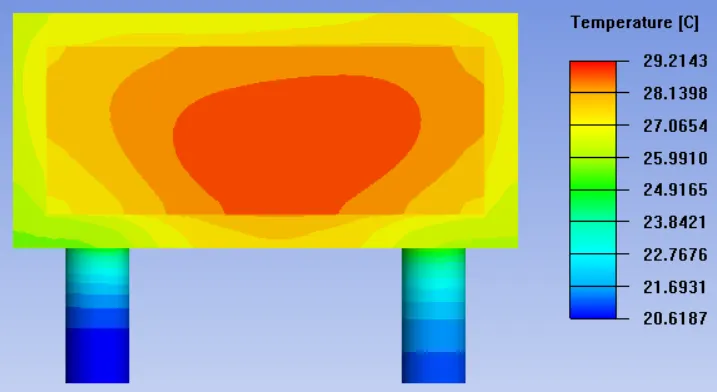
The image attached above shows the steady state temperature contours plotted on the outer faces of all the objects in the geometry that are defined as solid type.
According to contour plot, the maximum temperature (29.2143 degree C) is observed over the heated plates.
Velocity contours
The velocity contours are plotted along different cut-planes to observe the velocity distribution throughout the domain at steady state.
Velocity contours plotted on the Z-Plane through the center
The velocity contours below shows the steady state velocity contours plotted on the cut-plane passing through the center of the cabinet and perpendicular to Z-axis.
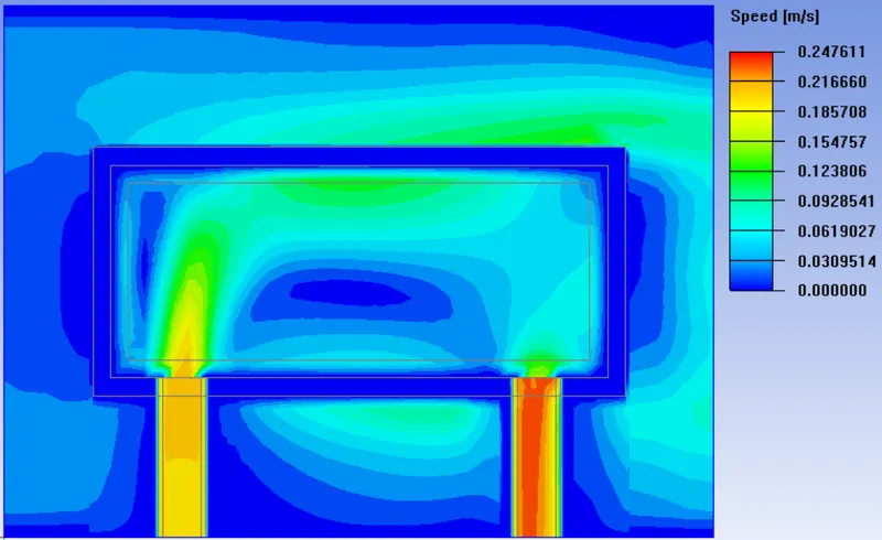
Velocity contours plotted on the Y-Plane through the center
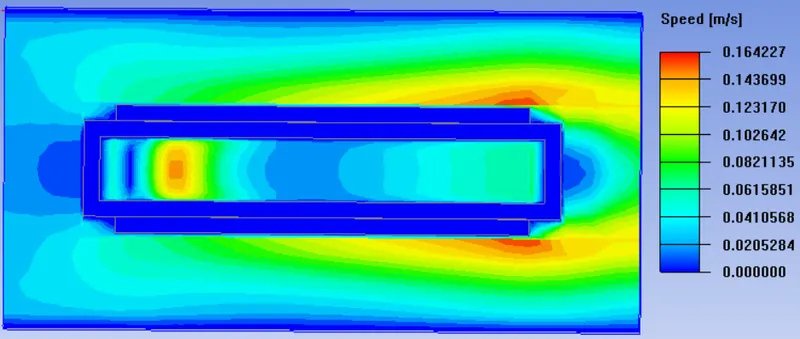
Velocity contours plotted on the X-Plane through the center
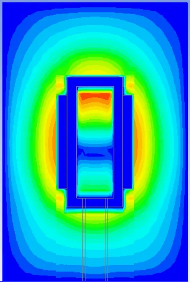
Velocity Vectors
The Velocity vectors are plotted along different cut-planes to gain further insight into the velocity distribution throughout the domain at steady state
Velocity vectors plotted on the Z plane through the center
The image attached below shows the steady state velocity vectors plotted on the cut-plane passing through the center of the cabinet and perpendicular to Z-axis.
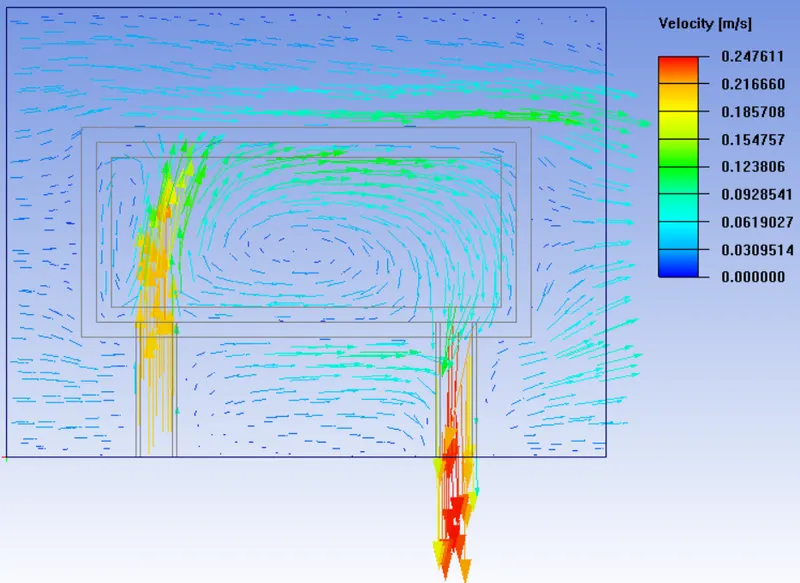
Velocity vectors plotted on the Y plane through the center
The image attached below shows the steady state velocity vectors plotted on the cut-plane passing through the center of the cabinet and perpendicular to Y-axis.
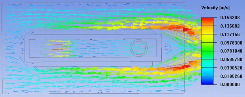
The vector plot shows that air accelerates as it moves up against gravity due to natural convection. The vector plot successfully captures the recirculation zone behind Solid_block but is unable to capture the convection cells observed in the velocity contour plot.
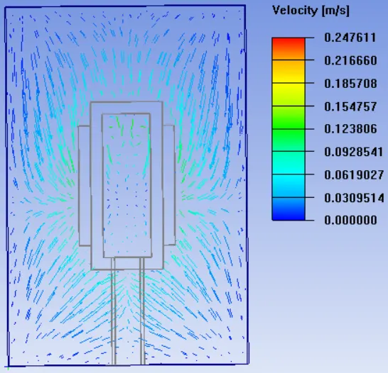
Velocity vectors plotted on the X plane through the center
The image attached below shows the steady state velocity vectors plotted on the cut-plane passing through the center of the cabinet and perpendicular to X-axis.
Conclusion
In the current project, CFD simulation of cold-plate cavity was performed using ANSYS Icepak. The model was created using the given design specifications. Non-cormal meshing was employed with local mesh refinement using object parameters. Zero equation turbulence model was employed to capture turbulance.
The gravity vector was defined along -X direction. Four surface probes were defined to monitor average temperature over four surfaces in the computational domain. The discretised governing equations were solved on the computational mesh for flow and temperature using Fluent solver engine.
1. Average temperature of air leaving the cabinet measured as 21 degree C and the average temperature of water leaving the cabinet was measured as 20.5 degree C.
2. According to the fluid face temperature contours, the maximum temperature (28.8301 degree C) is observed beneath the heated plates.
3.According to the solid face temperature contours, the maximum temperature (29.2143 degree C) is observed over the heated plates.