Week 3 - Solving second order ODEs
Governing Equation for Simple Pendulum with damping is derived from Newton's second law:
F = ma --(1)
Also, Net Force, F = restoring force + damping force
So,
F=ma = restoring force + damping force ---(1)
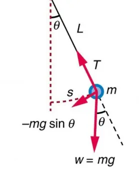
Distance travelled by pendulum is :
S=lθ ---(2)
Differenciating equation(2):
dS/dt = l*dθ/dt ---(3)
Differenciating equation(3):
dS^2/dt^2 = l*dθ^2/dt^2 ---(4) , accelaration
F=ma = restoring force + damping force ---(1)
Substitute eq(4) in (1)
m*l*dθ^2/dt^2 = restoring force + damping force
restoring force = -mgsinθ
damping force = -b*dθ/dt
m*l*dθ^2/dt^2 = -m*g*sinθ -b*dθ/dt
divide above equation with m*l on RHS and LHS
dθ^2/dt^2 = -(g/l)*sinθ -(bl)/(ml)*dθ/dt
dθ^2/dt^2 + (g/l)*sinθ + (b)/(m)*dθ/dt =0 -----(5)
In order to solve eq(5),2 order ODE simplify to below two equations of single order ODE
dθ1/dt = θ2
dθ2/dt = -(b/m)-(g/l)*sinθ1
MATLAB Code to solve above equations
--------------------------------------------------------------------------
clear all
close all
clc
% definine geometry details of pendulum
%damping co-efficient
b=0.05;
%gravity m/s^2
g=9.81;
%length of string in meters
l=1;
% mass of ball in kg
m=0.1;
% counter value used in for loop for animation purpose
ct=1;
%initial condition, initial displacement=0 @ velocity = 5 m/s
theta_0 =[0;5]
% time points. time span is for 0 to 10 seconds. 500 data points are calculated between 0 to 10 seconds
t_span=linspace(0,10,500);
% Solve ODE, "ode45" is buit-in function of MATLAB to solve ODE equations
% ode_func(t,theta,b,g,l,m) is sub-funnction written
[t,results]=ode45(@(t,theta) ode_func(t,theta,b,g,l,m), t_span, theta_0);
% plot Angular displacement and Angular Velocity
figure(1)
plot(t,results(:,1))
hold on
plot(t,results(:,2))
ylabel('plot')
xlabel('time')
legend('Angular Displacement','Angular Velocity')
grid on
% for loop for animation of simple pendulum
for i = 1:length(t_span)
x0=0;
y0=0;
% sin(x)-> x must be in radians and sind(x)-> x must be degrees
x1 = l*sind(results(i,1));
y1 = -l*cosd(results(i,1));
% Plotting
figure(2)
plot([x0,x1],[y0,y1],[-0.5 0.5],[0 0],'linewidth',3)
hold on
plot(x1,y1,'marker','o','markerSize',20,'markerFacecolor','y')
% axis cordinates reset on x-axis (-1.5 to 1.5) and y-axis (-0.5 to 0.5)
axis([-0.1 0.1 -1.5 0.5])
grid on
%Time between two successive plots on graph
pause(0.03)
% storing each image in M(cf) array, this is used to write movie file later
M(ct) = getframe(gcf);
% increment ct value
ct = ct+1;
hold off
end
-------------------------------------------------------------------------------------------
Sub function to calculate angular displacement and angular velocity
-------------------------------------------------------------------------------------------
function[dtheta_dt]=ode_func(t,theta,b,g,l,m)
theta1=theta(1)
theta2=theta(2)
dtheta1_dt=theta2;
dtheta2_dt=-(b/m)*theta2-(g/l)*sin(theta1);
dtheta_dt=[dtheta1_dt;dtheta2_dt];
end
-----------------------------------------------------------------------------------------------
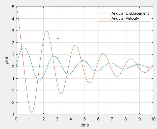
with damping value of b=0.05
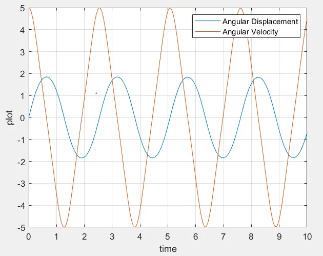
without damping, b=0
-----------------------------------------------------------------------------------------------
New learnings from this Project:
-----------------------------------------------------------------------------------------------
1. about "ode45" buit-in function in MATLAB
2. "figure(2) " command to plot graphs
3. "marker" sub option in "plot" used to create bob of simple pendulum :
plot(x1,y1,'marker','o','markerSize',20,'markerFacecolor','y')
----------------------------------------------------
Link for animation : https://youtu.be/2aeUeAhAQUQ
----------------------------------------------------