Curve fitting using MATLAB Code for provided data

Theory:curve fitting is a process of constructing a curve or mathematical function, that has best fit to a series of data points.

Based on the accuracy of curve fit the value of predicted data can change but we have an impression ofthe trend.

curve fitting funtions used in this assignment are :

1. Linear Equation -> y=ax+b

2. Quadratic Equation -> y=ax^2+b*X+c

3. Cubic Equation -> y=ax^3+b*x^2+c*x+d

Parameters used for curve fitting are:

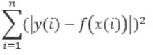
1. Sum of Squares due to errors (SSE)

It is square of error, where error or difference between predicted data and actual data

SSE (Sum of squared errors) :-

2. R-Square

R-Square of correlation between the response value and predicted value.

R-Square value ranges from 0 to 1.

Higher value of R-square will indicate better fit.

R^2 = SSR/SST

where SSR is :

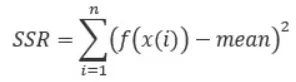
SST = SSR + SSE.

------------------------------------------------------------------------------------------------

MATLAB CODE

-------------------------------------------------------------------------------------------

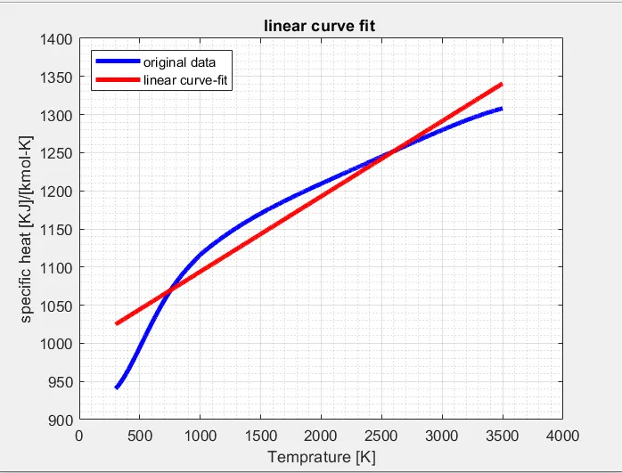
Linear Fit :

clear all
close all
clc

% load data from external file to variable

cp_data = load('data');

%first column is temperature and second column is specific heat

%assign temperature data to a variable "temp"
temp=cp_data(:,1);

%assign specific heat data to a variable "cp"
cp=cp_data(:,2);

% Linear curve fit : cp = a*T + b -> y=ax+b ; polyfit(x,y,1) while 1 represents linear fit. polyfit returns coefficients of equation.

co_effs=polyfit(temp,cp,1);

% polyval is function used to predict data using coefficients and x-axis values.

predicted_cp = polyval(co_effs,temp);

%compare quadratic curve fit with original data

plot(temp,cp,'linewidth',3,'color','b');
hold on

plot(temp,predicted_cp,'linewidth',3,'color','r');

axis([0 4000 900 1400]); % setting axis limits of graph axis([x1 x2 y1 y3)]
grid on;
grid minor;

xlabel('Temprature [K]');
ylabel('specific heat [KJ]/[kmol-K]')

legend('original data','linear curve-fit','Location','northwest');
title('linear curve fit ')

% Regression Analysis

summ = 0;
% To calculate mean of cp
% First step is to find sum of all the cp values by adding
% Second step is to divide the sum of cp by number of data points
for i=1:3200

summ=summ+cp_data(i,2)

end

mean = summ/3200;

% sum of squares of regression
ssr=0;
% sum of squared errors
sse=0;

for j=1:3200

ssr=ssr+(predicted_cp(j)-mean)^2;
sse=sse+(cp_data(j,2)-predicted_cp(j))^2;

end

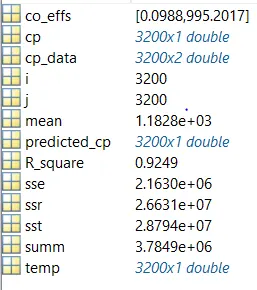
sst = ssr + sse ;
% Value of R_square indicates curve fit is good or not.
% Value of R_square closer to 1 is good fit.
R_square = ssr/sst;

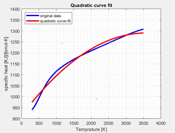
Square Fit :

clear all
close all
clc

% load data from external file to variable

cp_data = load('data');

%first column is temperature and second column is specific heat

%assign temperature data
temp=cp_data(:,1);

%assign specific heat data
cp=cp_data(:,2);

% Quadratic curve fit : cp = a*T^2 + b*T + C
%polyfit function returns co-efficients a,b,c values for above equation

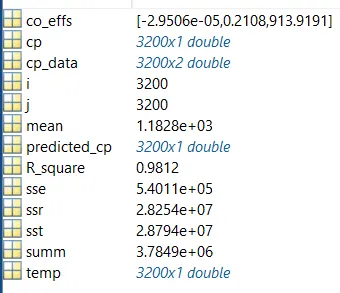
co_effs=polyfit(temp,cp,2);

predicted_cp = polyval(co_effs,temp);

%compare quadratic curve fit with original data

plot(temp,cp,'linewidth',3,'color','b');
hold on
plot(temp,predicted_cp,'linewidth',3,'color','r');

xlabel('Temprature [K]');
ylabel('specific heat [KJ]/[kmol-K]')

legend('original data','quadratic curve-fit','Location','northwest');
title('Quadratic curve fit')
axis([0 4000 900 1400]);
grid on;
grid minor;

% Regression Analysis

summ = 0;
% To calculate mean of cp
% First step is to find sum of all the cp values by adding
% Second step is to divide the sum of cp by number of data points
for i=1:3200

summ=summ+cp_data(i,2)

end

mean = summ/3200;

% sum of squares of regression
ssr=0;
% sum of squared errors
sse=0;

for j=1:3200

ssr=ssr+(predicted_cp(j)-mean)^2;
sse=sse+(cp_data(j,2)-predicted_cp(j))^2;

end

sst = ssr + sse ;
% Value of R_square indicates curve fit is good or not.
% Value of R_square closer to 1 is good fit.
R_square = ssr/sst;

Cubic Fit :

clear all
close all
clc

% load data from external file to variable

cp_data = load('data');

%first column is temperature and second column is specific heat

%assign temperature data
temp=cp_data(:,1);

%assign specific heat data
cp=cp_data(:,2);

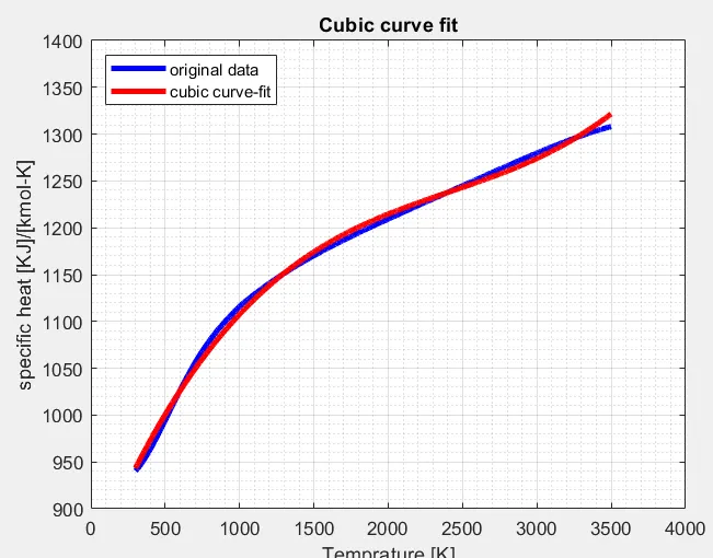
% Cubix curve fit : cp = a*T^3 + b*T^2 + C*T + d
%polyfit function returns co-efficients a,b,c values for above equation

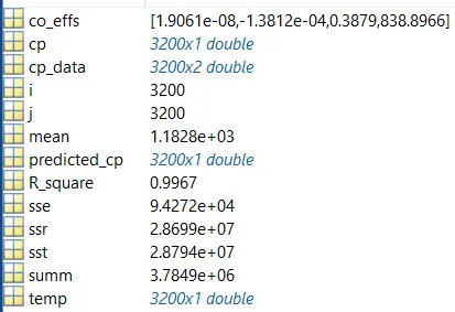
co_effs=polyfit(temp,cp,3);

predicted_cp = polyval(co_effs,temp);

%compare quadratic curve fit with original data

plot(temp,cp,'linewidth',3,'color','b');
hold on
plot(temp,predicted_cp,'linewidth',3,'color','r');

xlabel('Temprature [K]');
ylabel('specific heat [KJ]/[kmol-K]')

legend('original data','cubic curve-fit','Location','northwest');
title('Cubic curve fit')
axis([0 4000 900 1400]);
grid on;
grid minor;

% Regression Analysis

summ = 0;
% To calculate mean of cp
% First step is to find sum of all the cp values by adding
% Second step is to divide the sum of cp by number of data points
for i=1:3200

summ=summ+cp_data(i,2)

end

mean = summ/3200;

% sum of squares of regression
ssr=0;
% sum of squared errors
sse=0;

for j=1:3200

ssr=ssr+(predicted_cp(j)-mean)^2;
sse=sse+(cp_data(j,2)-predicted_cp(j))^2;

end

sst = ssr + sse ;
% Value of R_square indicates curve fit is good or not.
% Value of R_square closer to 1 is good fit.
R_square = ssr/sst;

Multiple Split Curve fit :

clear all
close all
clc

% load data from external file to variable

cp_data = load('data');

temp=cp_data(:,1);
cp=cp_data(:,2);

coeff1 = polyfit(temp(1:400),cp(1:400),1);
coeff2 = polyfit(temp(400:1200),cp(400:1200),2);
coeff3 = polyfit(temp(1200:3200),cp(1200:3200),1);

%calculate predicted Specific heat values

predicted_cp1=polyval(coeff1,temp(1:400));
predicted_cp2=polyval(coeff2,temp(400:1200));
predicted_cp3=polyval(coeff3,temp(1200:3200));

%plotting graph
plot(temp,cp,'linewidth',3.0,'color','r')

hold on

plot(temp(1:400),predicted_cp1,'linewidth',1.0,'color','c')
plot(temp(400:1200),predicted_cp2,'linewidth',1.0,'color','y')
plot(temp(1200:3200),predicted_cp3,'linewidth',1.0,'color','b')
axis([0 4000 900 1400]);
grid on;
grid minor;

hold off

xlabel('Temperature in K')
ylabel('specific heat in KJ/kmol-K')
title('splitwise curve fit data')
legend('Original data','Split1','split2','split3','location','northwest')

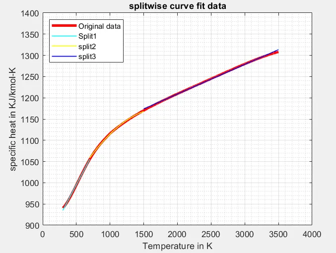
Using Curve fitting tool from MATLAB

	Code	Tool Box
Linear Fit	0.9249	0.9249
Square Fit	0.9812	0.9812
Cubic Fit	0.9967	0.9967

CONCLUSION

1. R^2 value is same between code and Tool box of MATLAB.

2. Split data : linear,square and linear equation has been used to predict data based on behaviour of original data.